Nontraditional Transportation Models

NONTRADITIONAL TRANSPORTATION MODELS

The application of the transportation model is not limited to transporting commodities between geographical sources and destinations. This section presents two applications in the areas of production-inventory control and tool sharpening service.

Example 5.2-1   (Production-Inventory Control)

Boralis manufactures backpacks for serious hikers. The demand for its product occurs during March to June of each year. Boralis estimates the demand for the four months to be 100, 200, 180, and 300 units, respectively. The company uses part-time labor to manufacture the backpacks and, accordingly, its production capacity varies monthly. It is estimated that Boralis can produce 50, 180,280, and 270 units in March through June. Because the production capacity and demand for the different months do not match, a current month's demand may be satisfied in one of three ways.

a)     Current month's production.

b)    Surplus production in an earlier month.

c)     Surplus production in a later month (backordering).

In the first case, the production cost per backpack is $40. The second case incurs an additional holding cost of $.50 per backpack per month. In the third case, an additional penalty cost of $2.00 per backpack is incurred for each month delay. Boralis wishes to determine the optimal production schedule for the four months.

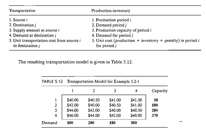
The situation can be modeled as a transportation model by recognizing the following parallels between the elements of the production-inventory problem and the transportation model:

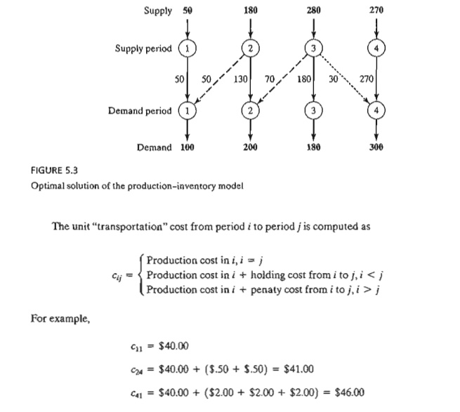
The optimal solution is summarized in Figure 5.3. The dashed lines indicate back-ordering, the dotted lines indicate production for a future period, and the solid lines show production in a period for itself. The total cost is $31,455.

Example 5.2-2              (Tool Sharpening)

Arkansas Pacific operates a medium-sized saw mill. The mill prepares different types of wood that range from soft pine to hard oak according to a weekly schedule. Depending on the type of wood being milled, the demand for sharp blades varies from day to day according to the follow-ing I-week (7-day) data:

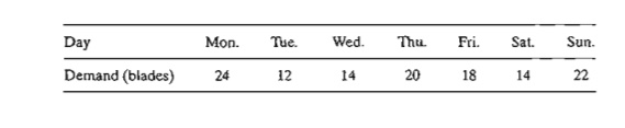
The mill can satisfy the daily demand in the following manner:

a)  Buy new blades at the cost of $12 a blade.

b)  Use an overnight sharpening service at the cost of $6 a blade.

c)   Use a slow 2-day sharpening service at the cost of $3 a blade.

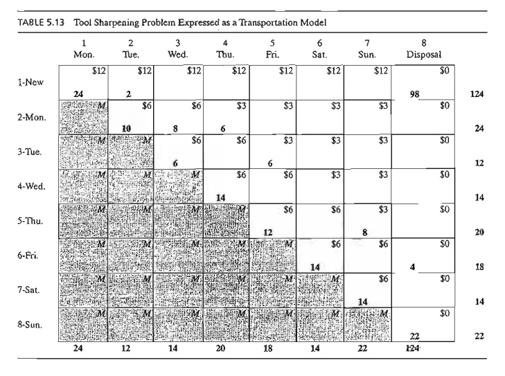
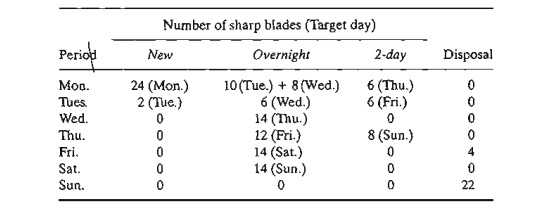
The situation can be represented as a transportation model with eight sources and seven destinations. The destinations represent the 7 days of the week. The sources of the model are defined as follows: Source 1 corresponds to buying new blades, which, in the extreme case, can provide sufficient supply to cover the demand for all 7 days (= 24 + 12 + 14 + 20 + 18 + 14 + 22 = 124). Sources 2 to 8 correspond to the 7 days of the week. The amount of supply for each of these sources equals the number of used blades at the end of the associated day. For ex-ample, source 2 (i.e., Monday) will have a supply of used blades equal to the demand for Mon-day. The unit "transportation cost" for the model is $12, $6, or $3, depending on whether the blade is supplied from new blades, overnight sharpening, or 2-day sharpening. Notice that the overnight service means that used blades sent at the end of day i will be available for use at the start of day i + 1 or day i + 2, because the slow 2-day service will not be available until the start of day i + 3. The "disposal" column is a dummy destination needed to balance the model. The com-plete model and its solution are given in Table 5.13.

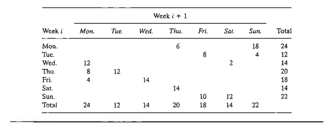
The problem has alternative optima at a cost of $840 (file toraExS.2-2.txt).The following table summarizes one such solution.

Remarks. The model in Table 5.13 is suitable only for the first week of operation because it does not take into account the rotational nature of the days of the week, in the sense that this week's days can act as sources for next week's demand. One way to handle this situation is to assume that the very first week of operation starts with all new blades for each day. From then on, we use a model consisting of exactly 7 sources and 7 destinations corresponding to the days of the week. The new model will be similar to Table 5.13 less source "New" and destination "Disposal." Also, only diagonal cells will be blocked (unit cost = M). The remaining cells will have a unit cost of either $3.00 or $6.00. For example, the unit cost for cell (Sat., Mon.) is $6.00 and that for cells (Sat., Tue.), (Sat., Wed.), (Sat., Thu.), and (Sat., Fri.) is $3.00. The table below gives the solution costing $372. As expected, the optimum solution will always use the 2-day service only. The problem has alternative optima (see file toraEx5.2-2a.txt).

PROBLEM SET S.2A

1. In Example 5.2-1, suppose that the holding cost per unit is period-dependent and is given by 40, 30, and 70 cents for periods 1,2, and 3, respectively. The penalty and production costs I'emain as given in the example. Determine the optimum solution and interpret the results.

*2. In Example 5.2-2, suppose that the sharpening service offers 3-day service for $1 a blade on Monday and Tuesday (days 1 and 2). Reformulate the problem, and interpret the opti-mum solution.

3. In Example 5.2-2, if a blade is not used the day it is sharpened, a holding cost of 50 cents per blade per day is incurred. Reformulate the model, and interpret the optimum solution.

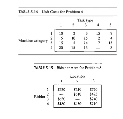
4. JoShop wants to assign four different categories of machines to five types of tasks. The numbers of machines available in the four categories are 25, 30,20, and 30. The numbers of jobs in the five tasks are 20, 20, 30,10, and 25. Machine category 4 cannot be assigned to task type 4. Table 5.14 provides the unit cost (in dollars) of assigning a machine cate-gory to a task type. The objective of the problem is to determine the optimum number of machines in each category to be assigned to each task type. Solve the problem and inter-pret the solution.

*5. The demand for a perishable item over the next four months is 400,300,420, and 380 tons, respectively. The supply capacities for the same months are 500, 600, 200, and 300 tons. The purchase price per ton varies from month to month and is estimated at $100, $140, $120, and $150, respectively. Because the item is perishable, a current month's sup-ply must be consumed within 3 months (starting with current month). The storage cost per ton per month is $3. The nature of the item does not allow back-ordering, Solve the problem as a transportation model and determine the optimum delivery schedule for the item over the next 4 months.

6. The demand for a special small engine over the next five quarters is 200, 150, 300,250, and 400 units. The manufacturer supplying the engine has different production capacities estimated at 180,230,430,300, and 300 for the five quarters. Back-ordering is not al-lowed, but the manufacturer may use overtime to fill the immediate demand, if necessary. The overtime capacity for each period is half the regular capacity. The production costs per unit for the five periods are $100, $96, $116, $102, and $106, respectively. TIle over-time production cost per engine is 50% higher than the regular production cost. If an en-gine is produced now for use in later periods, an additional storage cost of $4 per engine per period is incurred. Formulate the problem as a transportation model. Determine the optimum number of engines to be produced during regular time and overtime of each period.

7. Periodic preventive maintenance is carried out on aircraft engines, where an important component must be replaced. The numbers of aircraft scheduled for such maintenance over the next six months are estimated at 200, 180,300,198,230, and 290, respectively. All maintenance work is done during the first day of the month, where a used component may be replaced with a new or an overhauled component. The overhauling of used com-ponents may be done in a local repair facility, where they will be ready for use at the be-ginning of next month, or they may be sent to a central repair shop, where a delay of

3 months (including the month in which maintenance occurs) is expected. The repair cost in the local shop is $120 per component. At the central facility, the cost is only $35 per component. An overhauled component used in a later month will incur an additional storage cost of $1.50 per unit per month. New components may be purchased at $200 each in month 1, with a 5% price increase every 2 months. Formulate the problem as a transportation model, and determine the optimal schedule for satisfying the demand for the component over the next six months.

8. The National Parks Service is receiving four bids for logging at three pine forests in Arkansas. The three locations include 10,000,20,000, and 30,000 acres. A single bidder can bid for at most 50% of the total acreage available. The bids per acre at the three locations are given in Table 5.15. Bidder 2 does not wish to bid on location I, and bidder 3 cannot bid on location 2.

a. In the present situation, we need to maximize the total bidding revenue for the Parks Service. Show how the problem can be formulated as a transportation model.

b. Determine the acreage that should be assigned to each of the four bidders.