Temporal Database Concepts

Temporal Database Concepts

Temporal databases, in the broadest sense, encompass all database applications that require some aspect of time when organizing their information. Hence, they provide a good example to illustrate the need for developing a set of unifying concepts for application developers to use. Temporal database applications have been

developed since the early days of database usage. However, in creating these applications, it is mainly left to the application designers and developers to discover, design, program, and implement the temporal concepts they need. There are many examples of applications where some aspect of time is needed to maintain the information in a database. These include healthcare, where patient histories need to be maintained; insurance, where claims and accident histories are required as well as information about the times when insurance policies are in effect; reservation systems in general (hotel, airline, car rental, train, and so on), where information on the dates and times when reservations are in effect are required; scientific databases, where data collected from experiments includes the time when each data is measured; and so on. Even the two examples used in this book may be easily expanded into temporal applications. In the COMPANY database, we may wish to keep SALARY, JOB, and PROJECT histories on each employee. In the UNIVERSITY data-base, time is already included in the SEMESTER and YEAR of each SECTION of a COURSE, the grade history of a STUDENT, and the information on research grants. In fact, it is realistic to conclude that the majority of database applications have some temporal information. However, users often attempt to simplify or ignore temporal aspects because of the complexity that they add to their applications.

In this section, we will introduce some of the concepts that have been developed to deal with the complexity of temporal database applications. Section 26.2.1 gives an overview of how time is represented in databases, the different types of temporal information, and some of the different dimensions of time that may be needed. Section 26.2.2 discusses how time can be incorporated into relational databases. Section 26.2.3 gives some additional options for representing time that are possible in database models that allow complex-structured objects, such as object databases. Section 26.2.4 introduces operations for querying temporal databases, and gives a brief overview of the TSQL2 language, which extends SQL with temporal concepts. Section 26.2.5 focuses on time series data, which is a type of temporal data that is very important in practice.

1. Time Representation, Calendars, and Time Dimensions

For temporal databases, time is considered to be an ordered sequence of points in some granularity that is determined by the application. For example, suppose that some temporal application never requires time units that are less than one second. Then, each time point represents one second using this granularity. In reality, each second is a (short) time duration, not a point, since it may be further divided into milliseconds, microseconds, and so on. Temporal database researchers have used the term chronon instead of point to describe this minimal granularity for a particular application. The main consequence of choosing a minimum granularity—say, one second—is that events occurring within the same second will be considered to be simultaneous events, even though in reality they may not be.

Because there is no known beginning or ending of time, one needs a reference point from which to measure specific time points. Various calendars are used by various cultures (such as Gregorian (western), Chinese, Islamic, Hindu, Jewish, Coptic, and so on) with different reference points. A calendar organizes time into different time units for convenience. Most calendars group 60 seconds into a minute, 60 minutes into an hour, 24 hours into a day (based on the physical time of earth’s rotation around its axis), and 7 days into a week. Further grouping of days into months and months into years either follow solar or lunar natural phenomena, and are generally irregular. In the Gregorian calendar, which is used in most western countries, days are grouped into months that are 28, 29, 30, or 31 days, and 12 months are grouped into a year. Complex formulas are used to map the different time units to one another.

In SQL2, the temporal data types (see Chapter 4) include DATE (specifying Year, Month, and Day as YYYY-MM-DD), TIME (specifying Hour, Minute, and Second as HH:MM:SS), TIMESTAMP (specifying a Date/Time combination, with options for including subsecond divisions if they are needed), INTERVAL (a relative time duration, such as 10 days or 250 minutes), and PERIOD (an anchored time duration with a fixed starting point, such as the 10-day period from January 1, 2009, to January 10, 2009, inclusive).

Event Information versus Duration (or State) Information. A temporal data-base will store information concerning when certain events occur, or when certain facts are considered to be true. There are several different types of temporal information. Point events or facts are typically associated in the database with a single time point in some granularity. For example, a bank deposit event may be associated with the timestamp when the deposit was made, or the total monthly sales of a product (fact) may be associated with a particular month (say, February 2010). Note that even though such events or facts may have different granularities, each is still associated with a single time value in the database. This type of information is often represented as time series data as we will discuss in Section 26.2.5. Duration events or facts, on the other hand, are associated with a specific time period in the data-base. For example, an employee may have worked in a company from August 15, 2003 until November 20, 2008.

A time period is represented by its start and end time points [START-TIME, END-TIME]. For example, the above period is represented as [2003-08-15, 2008-11-20]. Such a time period is often interpreted to mean the set of all time points from start-time to end-time, inclusive, in the specified granularity. Hence, assuming day granularity, the period [2003-08-15, 2008-11-20] represents the set of all days from August 15, 2003, until November 20, 2008, inclusive.

Valid Time and Transaction Time Dimensions. Given a particular event or fact that is associated with a particular time point or time period in the database, the association may be interpreted to mean different things. The most natural interpretation is that the associated time is the time that the event occurred, or the period during which the fact was considered to be true in the real world. If this interpretation is used, the associated time is often referred to as the valid time. A temporal database using this interpretation is called a valid time database.

However, a different interpretation can be used, where the associated time refers to the time when the information was actually stored in the database; that is, it is the value of the system time clock when the information is valid in the system. In this case, the associated time is called the transaction time. A temporal database using this interpretation is called a transaction time database.

Other interpretations can also be intended, but these are considered to be the most common ones, and they are referred to as time dimensions. In some applications, only one of the dimensions is needed and in other cases both time dimensions are required, in which case the temporal database is called a bitemporal database. If other interpretations are intended for time, the user can define the semantics and program the applications appropriately, and it is called a user-defined time.

The next section shows how these concepts can be incorporated into relational databases, and Section 26.2.3 shows an approach to incorporate temporal concepts into object databases.

2. Incorporating Time in Relational Databases Using Tuple Versioning

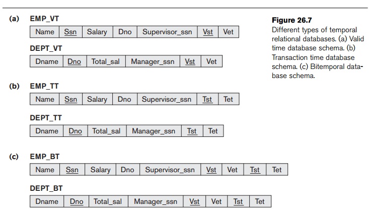
Valid Time Relations. Let us now see how the different types of temporal data-bases may be represented in the relational model. First, suppose that we would like to include the history of changes as they occur in the real world. Consider again the database in Figure 26.1, and let us assume that, for this application, the granularity is day. Then, we could convert the two relations EMPLOYEE and DEPARTMENT into valid time relations by adding the attributes Vst (Valid Start Time) and Vet (Valid End Time), whose data type is DATE in order to provide day granularity. This is shown in Figure 26.7(a), where the relations have been renamed EMP_VT and DEPT_VT, respectively.

Consider how the EMP_VT relation differs from the nontemporal EMPLOYEE relation (Figure 26.1). In EMP_VT, each tuple V represents a version of an employee’s

information that is valid (in the real world) only during the time period [V.Vst, V.Vet], whereas in EMPLOYEE each tuple represents only the current state or current version of each employee. In EMP_VT, the current version of each employee typically has a special value, now, as its valid end time. This special value, now, is a temporal variable that implicitly represents the current time as time progresses. The nontemporal EMPLOYEE relation would only include those tuples from the EMP_VT relation whose Vet is now.

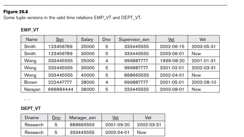
Figure 26.8 shows a few tuple versions in the valid-time relations EMP_VT and DEPT_VT. There are two versions of Smith, three versions of Wong, one version of Brown, and one version of Narayan. We can now see how a valid time relation should behave when information is changed. Whenever one or more attributes of an employee are updated, rather than actually overwriting the old values, as would happen in a nontemporal relation, the system should create a new version and close the current version by changing its Vet to the end time. Hence, when the user issued the command to update the salary of Smith effective on June 1, 2003, to $30000, the second version of Smith was created (see Figure 26.8). At the time of this update, the first version of Smith was the current version, with now as its Vet, but after the update now was changed to May 31, 2003 (one less than June 1, 2003, in day granularity), to indicate that the version has become a closed or history version and that the new (second) version of Smith is now the current one.

It is important to note that in a valid time relation, the user must generally provide the valid time of an update. For example, the salary update of Smith may have been entered in the database on May 15, 2003, at 8:52:12 A.M., say, even though the salary change in the real world is effective on June 1, 2003. This is called a proactive update, since it is applied to the database before it becomes effective in the real world. If the update is applied to the database after it becomes effective in the real world, it is called a retroactive update. An update that is applied at the same time as it becomes effective is called a simultaneous update.

The action that corresponds to deleting an employee in a nontemporal database would typically be applied to a valid time database by closing the current version of the employee being deleted. For example, if Smith leaves the company effective January 19, 2004, then this would be applied by changing Vet of the current version of Smith from now to 2004-01-19. In Figure 26.8, there is no current version for Brown, because he presumably left the company on 2002-08-10 and was logically deleted. However, because the database is temporal, the old information on Brown is still there.

The operation to insert a new employee would correspond to creating the first tuple version for that employee, and making it the current version, with the Vst being the effective (real world) time when the employee starts work. In Figure 26.7, the tuple on Narayan illustrates this, since the first version has not been updated yet.

Notice that in a valid time relation, the nontemporal key, such as Ssn in EMPLOYEE, is no longer unique in each tuple (version). The new relation key for EMP_VT is a combination of the nontemporal key and the valid start time attribute Vst, so we use (Ssn, Vst) as primary key. This is because, at any point in time, there should be at most one valid version of each entity. Hence, the constraint that any two tuple ver-sions representing the same entity should have nonintersecting valid time periods should hold on valid time relations. Notice that if the nontemporal primary key value may change over time, it is important to have a unique surrogate key attribute, whose value never changes for each real-world entity, in order to relate all versions of the same real-world entity.

Valid time relations basically keep track of the history of changes as they become effective in the real world. Hence, if all real-world changes are applied, the database keeps a history of the real-world states that are represented. However, because updates, insertions, and deletions may be applied retroactively or proactively, there is no record of the actual database state at any point in time. If the actual database states are important to an application, then one should use transaction time relations.

Transaction Time Relations. In a transaction time database, whenever a change is applied to the database, the actual timestamp of the transaction that applied the change (insert, delete, or update) is recorded. Such a database is most useful when changes are applied simultaneously in the majority of cases—for example, real-time stock trading or banking transactions. If we convert the nontemporal database in Figure 26.1 into a transaction time database, then the two relations EMPLOYEE and DEPARTMENT are converted into transaction time relations by adding the attributes Tst (Transaction Start Time) and Tet (Transaction End Time), whose data type is typically TIMESTAMP. This is shown in Figure 26.7(b), where the relations have been renamed EMP_TT and DEPT_TT, respectively.

In EMP_TT, each tuple V represents a version of an employee’s information that was created at actual time V.Tst and was (logically) removed at actual time V.Tet (because the information was no longer correct). In EMP_TT, the current version of each employee typically has a special value, uc (Until Changed), as its transaction end time, which indicates that the tuple represents correct information until it is changed by some other transaction. A transaction time database has also been called a rollback database, because a user can logically roll back to the actual database state at any past point in time T by retrieving all tuple versions V whose transaction time period [V.Tst, V.Tet] includes time point T.

Bitemporal Relations. Some applications require both valid time and transaction time, leading to bitemporal relations. In our example, Figure 26.7(c) shows how the EMPLOYEE and DEPARTMENT nontemporal relations in Figure 26.1 would appear as bitemporal relations EMP_BT and DEPT_BT, respectively. Figure 26.9 shows a few tuples in these relations. In these tables, tuples whose transaction end time Tet is uc are the ones representing currently valid information, whereas tuples whose Tet is an absolute timestamp are tuples that were valid until (just before) that timestamp. Hence, the tuples with uc in Figure 26.9 correspond to the valid time tuples in Figure 26.7. The transaction start time attribute Tst in each tuple is the timestamp of the transaction that created that tuple.

Now consider how an update operation would be implemented on a bitemporal relation. In this model of bitemporal databases, no attributes are physically changed in any tuple except for the transaction end time attribute Tet with a value of uc. To illustrate how tuples are created, consider the EMP_BT relation. The current version V of an employee has uc in its Tet attribute and now in its Vet attribute. If some attribute—say, Salary—is updated, then the transaction T that performs the update should have two parameters: the new value of Salary and the valid time VT when the new salary becomes effective (in the real world). Assume that VT− is the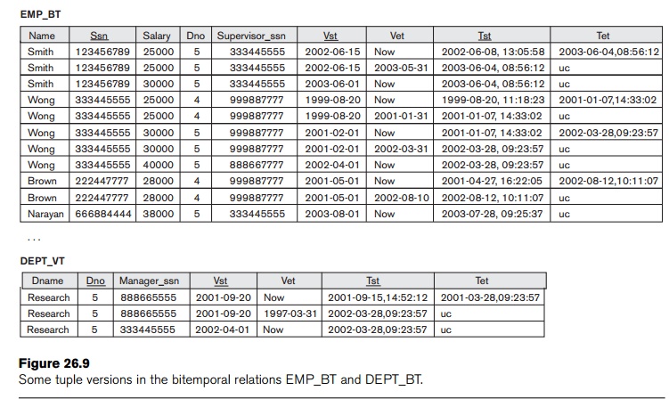

time point before VT in the given valid time granularity and that transaction T has a timestamp TS(T). Then, the following physical changes would be applied to the

EMP_BT table:

        1. Make a copy V₂ of the current version V; set V₂.Vet to VT−, V₂.Tst to TS(T), V₂.Tet to uc, and insert V₂ in EMP_BT; V₂ is a copy of the previous current version V after it is closed at valid time VT−.

        2. Make a copy V₃ of the current version V; set V₃.Vst to VT, V₃.Vet to now, V₃.Salary to the new salary value, V₃.Tst to TS(T), V₃.Tet to uc, and insert V₃ in EMP_BT; V₃ represents the new current version.

        3. Set V.Tet to TS(T) since the current version is no longer representing correct information.

As an illustration, consider the first three tuples V₁, V₂, and V₃ in EMP_BT in Figure 26.9. Before the update of Smith’s salary from 25000 to 30000, only V₁ was in EMP_BT and it was the current version and its Tet was uc. Then, a transaction T whose timestamp TS(T) is ‘2003-06-04,08:56:12’ updates the salary to 30000 with the effective valid time of ‘2003-06-01’. The tuple V₂ is created, which is a copy of V₁ except that its Vet is set to ‘2003-05-31’, one day less than the new valid time and its Tst is the timestamp of the updating transaction. The tuple V₃ is also created, which has the new salary, its Vst is set to ‘2003-06-01’, and its Tst is also the time-stamp of the updating transaction. Finally, the Tet of V₁ is set to the timestamp of the updating transaction, ‘2003-06-04,08:56:12’. Note that this is a retroactive update, since the updating transaction ran on June 4, 2003, but the salary change is effective on June 1, 2003.

Similarly, when Wong’s salary and department are updated (at the same time) to 30000 and 5, the updating transaction’s timestamp is ‘2001-01-07,14:33:02’ and the effective valid time for the update is ‘2001-02-01’. Hence, this is a proactive update because the transaction ran on January 7, 2001, but the effective date was February 1, 2001. In this case, tuple V₄ is logically replaced by V₅ and V₆.

Next, let us illustrate how a delete operation would be implemented on a bitemporal relation by considering the tuples V₉ and V₁₀ in the EMP_BT relation of Figure 26.9. Here, employee Brown left the company effective August 10, 2002, and the logical delete is carried out by a transaction T with TS(T) = 2002-08-12,10:11:07. Before this, V9 was the current version of Brown, and its Tet was uc. The logical delete is implemented by setting V₉.Tet to 2002-08-12,10:11:07 to invalidate it, and creating the final version V₁₀ for Brown, with its Vet = 2002-08-10 (see Figure 26.9). Finally, an insert operation is implemented by creating the first version as illustrated by V₁₁ in the EMP_BT table.

Implementation Considerations. There are various options for storing the tuples in a temporal relation. One is to store all the tuples in the same table, as shown in Figures 26.8 and 26.9. Another option is to create two tables: one for the currently valid information and the other for the rest of the tuples. For example, in the bitemporal EMP_BT relation, tuples with uc for their Tet and now for their Vet would be in one relation, the current table, since they are the ones currently valid (that is, represent the current snapshot), and all other tuples would be in another relation. This allows the database administrator to have different access paths, such as indexes for each relation, and keeps the size of the current table reasonable. Another possibility is to create a third table for corrected tuples whose Tet is not uc.

Another option that is available is to vertically partition the attributes of the tempo-ral relation into separate relations so that if a relation has many attributes, a whole new tuple version is created whenever any one of the attributes is updated. If the attributes are updated asynchronously, each new version may differ in only one of the attributes, thus needlessly repeating the other attribute values. If a separate rela-tion is created to contain only the attributes that always change synchronously, with the primary key replicated in each relation, the database is said to be in temporal normal form. However, to combine the information, a variation of join known as temporal intersection join would be needed, which is generally expensive to implement.

It is important to note that bitemporal databases allow a complete record of changes. Even a record of corrections is possible. For example, it is possible that two tuple versions of the same employee may have the same valid time but different attribute values as long as their transaction times are disjoint. In this case, the tuple with the later transaction time is a correction of the other tuple version. Even incor-rectly entered valid times may be corrected this way. The incorrect state of the data base will still be available as a previous database state for querying purposes. A data-base that keeps such a complete record of changes and corrections is sometimes called an append-only database.

3. Incorporating Time in Object-Oriented Databases Using Attribute Versioning

The previous section discussed the tuple versioning approach to implementing temporal databases. In this approach, whenever one attribute value is changed, a whole new tuple version is created, even though all the other attribute values will be identical to the previous tuple version. An alternative approach can be used in database systems that support complex structured objects, such as object data-bases (see Chapter 11) or object-relational systems. This approach is called attribute versioning.

In attribute versioning, a single complex object is used to store all the temporal changes of the object. Each attribute that changes over time is called a time-varying attribute, and it has its values versioned over time by adding temporal periods to the attribute. The temporal periods may represent valid time, transaction time, or bitemporal, depending on the application requirements. Attributes that do not change over time are called nontime-varying and are not associated with the temporal periods. To illustrate this, consider the example in Figure 26.10, which is an attribute-versioned valid time representation of EMPLOYEE using the object definition language (ODL) notation for object databases (see Chapter 11). Here, we assumed that name and Social Security number are nontime-varying attributes, whereas salary, department, and supervisor are time-varying attributes (they may change over time). Each time-varying attribute is represented as a list of tuples

<Valid_start_time, Valid_end_time, Value>, ordered by valid start time.

Whenever an attribute is changed in this model, the current attribute version is closed and a new attribute version for this attribute only is appended to the list. This allows attributes to change asynchronously. The current value for each attribute has now for its Valid_end_time. When using attribute versioning, it is useful to include a lifespan temporal attribute associated with the whole object whose value is one or more valid time periods that indicate the valid time of existence for the whole object. Logical deletion of the object is implemented by closing the lifespan. The constraint that any time period of an attribute within an object should be a subset of the object’s lifespan should be enforced.

For bitemporal databases, each attribute version would have a tuple with five components:

<Valid_start_time, Valid_end_time, Trans_start_time, Trans_end_time, Value>

The object lifespan would also include both valid and transaction time dimensions. Therefore, the full capabilities of bitemporal databases can be available with attribute versioning. Mechanisms similar to those discussed earlier for updating tuple versions can be applied to updating attribute versions.

class TEMPORAL_SALARY          

{        attribute      Date  Valid_start_time;

          attribute      Date  Valid_end_time;

          attribute      float  Salary;       

};                                   

class TEMPORAL_DEPT               

{        attribute      Date  Valid_start_time;

          attribute      Date  Valid_end_time;

          attribute      DEPARTMENT_VT     Dept;

};                                   

class TEMPORAL_SUPERVISOR           

{        attribute      Date  Valid_start_time;

          attribute      Date  Valid_end_time;

          attribute      EMPLOYEE_VT Supervisor;

};                                   

class TEMPORAL_LIFESPAN                 

{        attribute      Date  Valid_ start time;

          attribute      Date  Valid end time;

};                                   

class EMPLOYEE_VT           

(        extent EMPLOYEES  )          

{        attribute      list<TEMPORAL_LIFESPAN>        lifespan;

          attribute      string          Name;

          attribute      string          Ssn;

          attribute      list<TEMPORAL_SALARY> Sal_history;

          attribute      list<TEMPORAL_DEPT>      Dept_history;

          attribute      list <TEMPORAL_SUPERVISOR> Supervisor_history;

};                                   

Figure 26.10

Possible ODL schema for a temporal valid time EMPLOYEE_VT object class using attribute versioning.

4. Temporal Querying Constructs and the TSQL2 Language

So far, we have discussed how data models may be extended with temporal con-structs. Now we give a brief overview of how query operations need to be extended for temporal querying. We will briefly discuss the TSQL2 language, which extends SQL for querying valid time, transaction time, and bitemporal relational databases.

In nontemporal relational databases, the typical selection conditions involve attribute conditions, and tuples that satisfy these conditions are selected from the set of current tuples. Following that, the attributes of interest to the query are specified by a projection operation (see Chapter 6). For example, in the query to retrieve the names of all employees working in department 5 whose salary is greater than 30000, the selection condition would be as follows:

((Salary > 30000) AND (Dno = 5))

The projected attribute would be Name. In a temporal database, the conditions may involve time in addition to attributes. A pure time condition involves only time— for example, to select all employee tuple versions that were valid on a certain time point T or that were valid during a certain time period [T₁, T₂]. In this case, the specified time period is compared with the valid time period of each tuple version [T.Vst, T.Vet], and only those tuples that satisfy the condition are selected. In these operations, a period is considered to be equivalent to the set of time points from T₁ to T₂ inclusive, so the standard set comparison operations can be used. Additional operations, such as whether one time period ends before another starts are also needed.

Some of the more common operations used in queries are as follows:

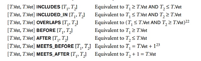
Additionally, operations are needed to manipulate time periods, such as computing the union or intersection of two time periods. The results of these operations may not themselves be periods, but rather temporal elements—a collection of one or more disjoint time periods such that no two time periods in a temporal element are directly adjacent. That is, for any two time periods [T₁, T₂] and [T₃, T₄] in a tempo-ral element, the following three conditions must hold:

        [T₁, T₂] intersection [T₃, T₄] is empty.

       T₃ is not the time point following T₂ in the given granularity. 

        T₁ is not the time point following T₄ in the given granularity.

The latter conditions are necessary to ensure unique representations of temporal elements. If two time periods [T₁, T₂] and [T₃, T₄] are adjacent, they are combined into a single time period [T₁, T₄]. This is called coalescing of time periods. Coalescing also combines intersecting time periods.

To illustrate how pure time conditions can be used, suppose a user wants to select all employee versions that were valid at any point during 2002. The appropriate selec-tion condition applied to the relation in Figure 26.8 would be

[T.Vst, T.Vet] OVERLAPS [2002-01-01, 2002-12-31]

Typically, most temporal selections are applied to the valid time dimension. For a bitemporal database, one usually applies the conditions to the currently correct tuples with uc as their transaction end times. However, if the query needs to be applied to a previous database state, an AS_OF T clause is appended to the query, which means that the query is applied to the valid time tuples that were correct in the database at time T.

In addition to pure time conditions, other selections involve attribute and time conditions. For example, suppose we wish to retrieve all EMP_VT tuple versions T for employees who worked in department 5 at any time during 2002. In this case, the condition is

[T.Vst, T.Vet]OVERLAPS [2002-01-01, 2002-12-31] AND (T.Dno = 5)

Finally, we give a brief overview of the TSQL2 query language, which extends SQL with constructs for temporal databases. The main idea behind TSQL2 is to allow users to specify whether a relation is nontemporal (that is, a standard SQL relation) or temporal. The CREATE TABLE statement is extended with an optional AS clause to allow users to declare different temporal options. The following options are avail-able:

        <AS VALID STATE <GRANULARITY> (valid time relation with valid time period)

        <AS VALID EVENT <GRANULARITY> (valid time relation with valid time point)

        <AS TRANSACTION (transaction time relation with transaction time period)

        <AS VALID STATE <GRANULARITY> AND TRANSACTION (bitemporal rela-tion, valid time period)

        <AS VALID EVENT <GRANULARITY> AND TRANSACTION (bitemporal rela-tion, valid time point)

The keywords STATE and EVENT are used to specify whether a time period or time point is associated with the valid time dimension. In TSQL2, rather than have the user actually see how the temporal tables are implemented (as we discussed in the previous sections), the TSQL2 language adds query language constructs to specify various types of temporal selections, temporal projections, temporal aggregations, transformation among granularities, and many other concepts. The book by Snodgrass et al. (1995) describes the language.

5. Time Series Data

Time series data is used very often in financial, sales, and economics applications. They involve data values that are recorded according to a specific predefined sequence of time points. Therefore, they are a special type of valid event data, where the event time points are predetermined according to a fixed calendar. Consider the example of closing daily stock prices of a particular company on the New York Stock Exchange. The granularity here is day, but the days that the stock market is open are known (nonholiday weekdays). Hence, it has been common to specify a computational procedure that calculates the particular calendar associated with a time series. Typical queries on time series involve temporal aggregation over higher granularity intervals—for example, finding the average or maximum weekly closing stock price or the maximum and minimum monthly closing stock price from the daily information.

As another example, consider the daily sales dollar amount at each store of a chain of stores owned by a particular company. Again, typical temporal aggregates would be retrieving the weekly, monthly, or yearly sales from the daily sales information (using the sum aggregate function), or comparing same store monthly sales with previous monthly sales, and so on.

Because of the specialized nature of time series data and the lack of support for it in older DBMSs, it has been common to use specialized time series management systems rather than general-purpose DBMSs for managing such information. In such systems, it has been common to store time series values in sequential order in a file, and apply specialized time series procedures to analyze the information. The problem with this approach is that the full power of high-level querying in languages such as SQL will not be available in such systems.

More recently, some commercial DBMS packages are offering time series extensions, such as the Oracle time cartridge and the time series data blade of Informix Universal Server. In addition, the TSQL2 language provides some support for time series in the form of event tables.