Spatial Database Concepts

Spatial Database Concepts

1. Introduction to Spatial Databases

Spatial databases incorporate functionality that provides support for databases that keep track of objects in a multidimensional space. For example, cartographic data-bases that store maps include two-dimensional spatial descriptions of their objects—from countries and states to rivers, cities, roads, seas, and so on. The systems that manage geographic data and related applications are known as Geographical Information Systems (GIS), and they are used in areas such as environmental applications, transportation systems, emergency response systems, and battle management. Other databases, such as meteorological databases for weather information, are three-dimensional, since temperatures and other meteorological information are related to three-dimensional spatial points. In general, a spatial database stores objects that have spatial characteristics that describe them and that have spatial relationships among them. The spatial relationships among the objects are important, and they are often needed when querying the database. Although a spatial database can in general refer to an n-dimensional space for any n, we will limit our discussion to two dimensions as an illustration.

A spatial database is optimized to store and query data related to objects in space, including points, lines and polygons. Satellite images are a prominent example of spatial data. Queries posed on these spatial data, where predicates for selection deal with spatial parameters, are called spatial queries. For example, “What are the names of all bookstores within five miles of the College of Computing building at Georgia Tech?” is a spatial query. Whereas typical databases process numeric and character data, additional functionality needs to be added for databases to process spatial data types. A query such as “List all the customers located within twenty miles of company headquarters” will require the processing of spatial data types typically outside the scope of standard relational algebra and may involve consult-ing an external geographic database that maps the company headquarters and each customer to a 2-D map based on their address. Effectively, each customer will be associated to a <latitude, longitude> position. A traditional B⁺-tree index based on customers’ zip codes or other nonspatial attributes cannot be used to process this query since traditional indexes are not capable of ordering multidimensional coordinate data. Therefore, there is a special need for databases tailored for handling spatial data and spatial queries.

Table 26.1 shows the common analytical operations involved in processing geographic or spatial data. Measurement operations are used to measure some

Table 26.1 Common Types of Analysis for Spatial Data

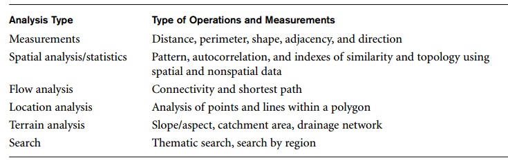
Analysis Type : Type of Operations and Measurements

Measurements : Distance, perimeter, shape, adjacency, and direction

Spatial analysis/statistics : Pattern, autocorrelation, and indexes of similarity and topology using spatial and nonspatial data

Flow analysis : Connectivity and shortest path

Location analysis : Analysis of points and lines within a polygon

Terrain analysis : Slope/aspect, catchment area, drainage network

Search : Thematic search, search by region

global properties of single objects (such as the area, the relative size of an object’s parts, compactness, or symmetry), and to measure the relative position of different objects in terms of distance and direction. Spatial analysis operations, which often use statistical techniques, are used to uncover spatial relationships within and among mapped data layers. An example would be to create a map—known as a prediction map—that identifies the locations of likely customers for particular products based on the historical sales and demographic information. Flow analysis operations help in determining the shortest path between two points and also the connectivity among nodes or regions in a graph. Location analysis aims to find if the given set of points and lines lie within a given polygon (location). The process involves generating a buffer around existing geographic features and then identifying or selecting features based on whether they fall inside or outside the boundary of the buffer. Digital terrain analysis is used to build three-dimensional models, where the topography of a geographical location can be represented with an x, y, z data model known as Digital Terrain (or Elevation) Model (DTM/DEM). The x and y dimensions of a DTM represent the horizontal plane, and z represents spot heights for the respective x, y coordinates. Such models can be used for analysis of environmental data or during the design of engineering projects that require terrain information. Spatial search allows a user to search for objects within a particular spatial region. For example, thematic search allows us to search for objects related to a particular theme or class, such as “Find all water bodies within 25 miles of Atlanta” where the class is water.

There are also topological relationships among spatial objects. These are often used in Boolean predicates to select objects based on their spatial relationships. For example, if a city boundary is represented as a polygon and freeways are represented as multilines, a condition such as “Find all freeways that go through Arlington, Texas” would involve an intersects operation, to determine which freeways (lines) intersect the city boundary (polygon).

2. Spatial Data Types and Models

This section briefly describes the common data types and models for storing spatial data. Spatial data comes in three basic forms. These forms have become a de facto standard due to their wide use in commercial systems.

Map Data includes various geographic or spatial features of objects in a map, such as an object’s shape and the location of the object within the map. The three basic types of features are points, lines, and polygons (or areas). Points are used to represent spatial characteristics of objects whose locations correspond to a single 2-d coordinate (x, y, or longitude/latitude) in the scale of a particular application. Depending on the scale, some examples of point objects could be buildings, cellular towers, or stationary vehicles. Moving vehicles and other moving objects can be represented by a sequence of point locations that change over time. Lines represent objects having length, such as roads or rivers, whose spatial characteristics can be approximated by a sequence of connected lines. Polygons are used to represent spatial characteristics of objects that have a boundary, such as countries, states, lakes, or cities. Notice that some objects, such as buildings or cities, can be represented as either points or polygons, depending on the scale of detail.

        Attribute data is the descriptive data that GIS systems associate with map features. For example, suppose that a map contains features that represent counties within a US state (such as Texas or Oregon). Attributes for each county feature (object) could include population, largest city/town, area in square miles, and so on. Other attribute data could be included for other features in the map, such as states, cities, congressional districts, census tracts, and so on.

        Image data includes data such as satellite images and aerial photographs, which are typically created by cameras. Objects of interest, such as buildings and roads, can be identified and overlaid on these images. Images can also be attributes of map features. One can add images to other map features so that clicking on the feature would display the image. Aerial and satellite images are typical examples of raster data.

Models of spatial information are sometimes grouped into two broad categories: field and object. A spatial application (such as remote sensing or highway traffic con-trol) is modeled using either a field- or an object-based model, depending on the requirements and the traditional choice of model for the application. Field models are often used to model spatial data that is continuous in nature, such as terrain ele-vation, temperature data, and soil variation characteristics, whereas object models have traditionally been used for applications such as transportation networks, land parcels, buildings, and other objects that possess both spatial and non-spatial attributes.

3. Spatial Operators

Spatial operators are used to capture all the relevant geometric properties of objects embedded in the physical space and the relations between them, as well as to perform spatial analysis. Operators are classified into three broad categories.

Topological operators. Topological properties are invariant when topological transformations are applied. These properties do not change after trans-formations like rotation, translation, or scaling. Topological operators are hierarchically structured in several levels, where the base level offers opera-tors the ability to check for detailed topological relations between regions with a broad boundary, and the higher levels offer more abstract operators that allow users to query uncertain spatial data independent of the underlying geometric data model. Examples include open (region), close (region), and inside (point, loop).

        Projective operators. Projective operators, such as convex hull, are used to express predicates about the concavity/convexity of objects as well as other spatial relations (for example, being inside the concavity of a given object).

        Metric operators. Metric operators provide a more specific description of the object’s geometry. They are used to measure some global properties of single objects (such as the area, relative size of an object’s parts, compactness, and symmetry), and to measure the relative position of different objects in terms of distance and direction. Examples include length (arc) and distance (point, point).

Dynamic Spatial Operators. The operations performed by the operators mentioned above are static, in the sense that the operands are not affected by the application of the operation. For example, calculating the length of the curve has no effect on the curve itself. Dynamic operations alter the objects upon which the operations act. The three fundamental dynamic operations are create, destroy, and update. A representative example of dynamic operations would be updating a spatial object that can be subdivided into translate (shift position), rotate (change orientation), scale up or down, reflect (produce a mirror image), and shear (deform).

Spatial Queries. Spatial queries are requests for spatial data that require the use of spatial operations. The following categories illustrate three typical types of spatial queries:

        Range query. Finds the objects of a particular type that are within a given spatial area or within a particular distance from a given location. (For exam-ple, find all hospitals within the Metropolitan Atlanta city area, or find all ambulances within five miles of an accident location.)

        Nearest neighbor query. Finds an object of a particular type that is closest to a given location. (For example, find the police car that is closest to the location of crime.)

        Spatial joins or overlays. Typically joins the objects of two types based on some spatial condition, such as the objects intersecting or overlapping spatially or being within a certain distance of one another. (For example, find all townships located on a major highway between two cities or find all homes that are within two miles of a lake.)

4. Spatial Data Indexing

A spatial index is used to organize objects into a set of buckets (which correspond to pages of secondary memory), so that objects in a particular spatial region can be easily located. Each bucket has a bucket region, a part of space containing all objects stored in the bucket. The bucket regions are usually rectangles; for point data structures, these regions are disjoint and they partition the space so that each point belongs to precisely one bucket. There are essentially two ways of providing a spatial index.

        Specialized indexing structures that allow efficient search for data objects

based on spatial search operations are included in the database system. These indexing structures would play a similar role to that performed by B⁺-tree indexes in traditional database systems. Examples of these indexing structures are grid files and R-trees. Special types of spatial indexes, known as spatial join indexes, can be used to speed up spatial join operations.

        Instead of creating brand new indexing structures, the two-dimensional

(2-d) spatial data is converted to single-dimensional (1-d) data, so that traditional indexing techniques (B⁺-tree) can be used. The algorithms for converting from 2-d to 1-d are known as space filling curves. We will not discuss these methods in detail (see the Selected Bibliography for further references).

We give an overview of some of the spatial indexing techniques next.

Grid Files. We introduced grid files for indexing of data on multiple attributes in Chapter 18. They can also be used for indexing 2-dimensional and higher n-dimensional spatial data. The fixed-grid method divides an n-dimensional hyper-space into equal size buckets. The data structure that implements the fixed grid is an n-dimensional array. The objects whose spatial locations lie within a cell (totally or partially) can be stored in a dynamic structure to handle overflows. This structure is useful for uniformly distributed data like satellite imagery. However, the fixed-grid structure is rigid, and its directory can be sparse and large.

R-Trees. The R-tree is a height-balanced tree, which is an extension of the B⁺-tree for k-dimensions, where k > 1. For two dimensions (2-d), spatial objects are approximated in the R-tree by their minimum bounding rectangle (MBR), which is the smallest rectangle, with sides parallel to the coordinate system (x and y) axis, that contains the object. R-trees are characterized by the following properties, which are similar to the properties for B⁺-trees (see Section 18.3) but are adapted to 2-d spatial objects. As in Section 18.3, we use M to indicate the maximum number of entries that can fit in an R-tree node.

        The structure of each index entry (or index record) in a leaf node is (I, object-identifier), where I is the MBR for the spatial object whose identifier is object-identifier.

        Every node except the root node must be at least half full. Thus, a leaf node that is not the root should contain m entries (I, object-identifier) where M/2 <= m <= M. Similarly, a non-leaf node that is not the root should contain m entries (I, child-pointer) where M/2 <= m <= M, and I is the MBR that contains the union of all the rectangles in the node pointed at by child-pointer.

        All leaf nodes are at the same level, and the root node should have at least two pointers unless it is a leaf node.

All MBRs have their sides parallel to the axes of the global coordinate system.

Other spatial storage structures include quadtrees and their variations. Quadtrees generally divide each space or subspace into equally sized areas, and proceed with the subdivisions of each subspace to identify the positions of various objects. Recently, many newer spatial access structures have been proposed, and this area remains an active research area.

Spatial Join Index. A spatial join index precomputes a spatial join operation and stores the pointers to the related object in an index structure. Join indexes improve the performance of recurring join queries over tables that have low update rates. Spatial join conditions are used to answer queries such as “Create a list of highway-river combinations that cross.” The spatial join is used to identify and retrieve these pairs of objects that satisfy the cross spatial relationship. Because computing the results of spatial relationships is generally time consuming, the result can be com-puted once and stored in a table that has the pairs of object identifiers (or tuple ids) that satisfy the spatial relationship, which is essentially the join index.

A join index can be described by a bipartite graph G = (V1,V2,E), where V1 contains the tuple ids of relation R, and V2 contains the tuple ids of relation S. Edge set contains an edge (vr,vs) for vr in R and vs in S, if there is a tuple corresponding to (vr,vs) in the join index. The bipartite graph models all of the related tuples as connected vertices in the graphs. Spatial join indexes are used in operations (see Section 26.3.3) that involve computation of relationships among spatial objects.

5. Spatial Data Mining

Spatial data tends to be highly correlated. For example, people with similar characteristics, occupations, and backgrounds tend to cluster together in the same neighborhoods.

The three major spatial data mining techniques are spatial classification, spatial association, and spatial clustering.

        Spatial classification. The goal of classification is to estimate the value of an attribute of a relation based on the value of the relation’s other attributes. An example of the spatial classification problem is determining the locations of nests in a wetland based on the value of other attributes (for example, vegetation durability and water depth); it is also called the location prediction problem. Similarly, where to expect hotspots in crime activity is also a location prediction problem.

        Spatial association. Spatial association rules are defined in terms of spatial predicates rather than items. A spatial association rule is of the form

P₁ ^ P₂ ^ ... ^ P_n ⇒ Q₁ ^ Q₂ ^ ...  ^ Q_m,

where at least one of the P_i’s or Q _j’s is a spatial predicate. For example, the rule

is_a(x, country) ^ touches(x, Mediterranean) ⇒ is_a (x, wine-exporter)

(that is, a country that is adjacent to the Mediterranean Sea is typically a wine exporter) is an example of an association rule, which will have a certain support s and confidence c.

Spatial colocation rules attempt to generalize association rules to point to collection data sets that are indexed by space. There are several crucial differences between spatial and nonspatial associations including:

        The notion of a transaction is absent in spatial situations, since data is embedded in continuous space. Partitioning space into transactions would lead to an overestimate or an underestimate of interest measures, for exam-ple, support or confidence.

        Size of item sets in spatial databases is small, that is, there are many fewer items in the item set in a spatial situation than in a nonspatial situation.

In most instances, spatial items are a discrete version of continuous variables. For example, in the United States income regions may be defined as regions where the mean yearly income is within certain ranges, such as, below $40,000, from $40,000 to $100,000, and above $100,000.

            Spatial Clustering attempts to group database objects so that the most similar objects are in the same cluster, and objects in different clusters are as dis-similar as possible. One application of spatial clustering is to group together seismic events in order to determine earthquake faults. An example of a spatial clustering algorithm is density-based clustering, which tries to find clusters based on the density of data points in a region. These algorithms treat clusters as dense regions of objects in the data space. Two variations of these algorithms are density-based spatial clustering of applications with noise (DBSCAN) and density-based clustering (DENCLUE). DBSCAN is a density-based clustering algorithm because it finds a number of clusters starting from the estimated density distribution of corresponding nodes.

6. Applications of Spatial Data

Spatial data management is useful in many disciplines, including geography, remote sensing, urban planning, and natural resource management. Spatial database management is playing an important role in the solution of challenging scientific problems such as global climate change and genomics. Due to the spatial nature of genome data, GIS and spatial database management systems have a large role to play in the area of bioinformatics. Some of the typical applications include pattern recognition (for example, to check if the topology of a particular gene in the genome is found in any other sequence feature map in the database), genome browser development, and visualization maps. Another important application area of spatial data mining is the spatial outlier detection. A spatial outlier is a spatially referenced object whose nonspatial attribute values are significantly different from those of other spatially referenced objects in its spatial neighborhood. For example, if a neighborhood of older houses has just one brand-new house, that house would be an outlier based on the nonspatial attribute ‘house_age’. Detecting spatial outliers is useful in many applications of geographic information systems and spatial data-bases. These application domains include transportation, ecology, public safety, public health, climatology, and location-based services.