Statistical analysis and experimental design - Nutrition Research Methodology

Statistical analysis and experimental design

In all areas of research, statistical analysis of results and data plays a pivotal role. This section is intended to give students some of the very basic concepts of statistics as it relates to research methodology.

Validity

Validity describes the degree to which the inference drawn from a study is warranted when account is taken of the study methods, the representativeness of the study sample and the nature of its source popula-tion. Validity can be divided into internal validity and external validity. Internal validity refers to the subjects actually sampled. External validity refers to the exten-sion of the findings from the sample to a target population.

Accuracy

Accuracy is a term used to describe the extent to which a measurement is close to the true value, and

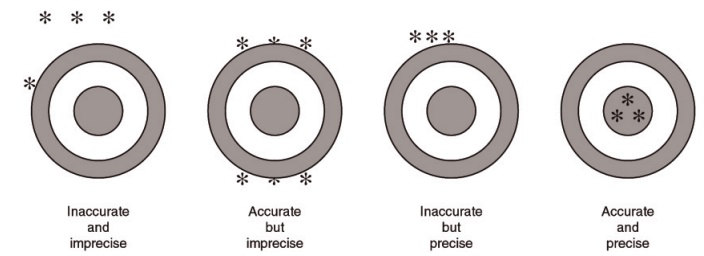
Figure 13.1 Accuracy and precision.

it is commonly estimated as the difference between the reported result and the actual value (Figure 13.1).

Reliability

Reliability or reproducibility refers to the consistency or repeatability of a measure. Reliability does not imply validity. A reliable measure is measuring some-thing consistently, but not necessarily estimating its true value. If a measurement error occurs in two sepa-rate measurements with exactly the same magnitude and direction, this measurement may be fully reliable but invalid. The kappa inter-rate agreement statistic (for categorical variables) and the intraclass cor-relation coefficient are frequently used to assess reliability.

Precision

Precision is described as the quality of being sharply defined or stated; thus, sometimes precision is indi-cated by the number of significant digits in the measurement.

In a more restricted statistical sense, precision refers to the reduction in random error. It can be improved either by increasing the size of a study or by using a design with higher efficiency. For example, a better balance in the allocation of exposed and unexposed subjects, or a closer matching in a case– control study usually obtains a higher precision without increasing the size of the study.

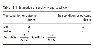
Sensitivity and specificity

Measures of sensitivity and specificity relate to the validity of a value. Sensitivity is the proportion of subjects with the condition who are correctly classified as having the condition. Specificity is the proportion of persons without the condition who are correctly classified as being free of the condition by the test or criteria. Sensitivity reflects the proportion of affected individuals who test positive, while speci-ficity refers to the proportion of nonaffected individ-uals who test negative (Table 13.1).

Data description

Statistics may have either a descriptive or an inferen-tial role in nutrition research. Descriptive statistical methods are a powerful tool to summarize large amounts of data. These descriptive purposes are served either by calculating statistical indices, such as the mean, median, and standard deviation, or by using graphical procedures, such as histograms, box plots, and scatter plots. Some errors in the data col-lection are most easily detected graphically with the histogram plot or with the box-plot chart (box-and-whisker plot). These two graphs are useful for describ-ing the distribution of a quantitative variable. Nominal variables, such as gender, and ordinal variables, such as educational level, can be presented simply tabulated as proportions within categories or ranks. Continuous variables, such as age and weight, are customarily presented by summary statistics describ-ing the frequency distribution. These summary statis-tics include measures of central tendency (mean, median) and measures of spread (variance, standard deviation, coefficient of variation). The standard deviation describes the “spread” or variation around the sample mean.

Hypothesis testing

The first step in hypothesis testing is formulating a hypothesis called the null hypothesis. This null hypothesis can often be stated as the negation of the research hypothesis that the investigator is looking for. For example, if we are interested in showing that, in the European adult population, a lower amount and intensity of physical activity during leisure time has contributed to a higher prevalence of overweight and obesity, the research hypothesis might be that there is a difference between sedentary and active adults with respect to their body mass index (BMI). The negation of this research hypothesis is called the null hypothesis. This null hypothesis simply main-tains that the difference in BMI between sedentary and active individuals is zero. In a second step, we calculate the probability that the result could have been obtained if the null hypothesis were true in the population from which the sample has been extracted. This probability is usually called the p-value. Its maximum value is 1 and the minimum is 0. The p-value is a conditional probability:

p-Value = prob(differences ≥ differences found | null hypothesis (H0) were true)

where the vertical bar (|) means “conditional to.” In a more concise mathematical expression:

p-Value = prob(difference ≥ data | H0)

The above condition is that the null hypothesis was true in the population that gave origin to the sample. The p-value by no means expresses the probability that the null hypothesis is true. This is a frequent and unfortunate mistake in the interpretation of p-values.

Hypothesis testing helps in deciding whether or not the null hypothesis can be rejected. A low p-value indicates that the data are not likely to be compatible with the null hypothesis. 

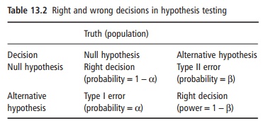
A large p-value indicates that the data are compatible with the null hypothesis. Many authors accept that a p-value lower than 0.05 provides enough evidence to reject the null hypothesis. The use of such a cut-off for p leads to treating the analysis as a decision-making process. Two possible errors can be made when making such a decision (Table 13.2).

A type I error consists of rejecting the null hypoth-esis, when the null hypothesis is in fact true. Con-versely, a type II error occurs if the null hypothesis is accepted when the null hypothesis is in fact not true. The probabilities of type I and type II errors are called alpha (α) and beta (β), respectively.

Power calculations

The power of a study is the probability of obtaining a statistically significant result when a true effect of a specified size exists. The power of a study is not a single value, but a range of values, depending on the assumption about the size of the effect. The plot of power against size of effect is called a power curve. The calculations of sample size are based in the prin-ciples of hypothesis testing. Thus, the power of a study to detect an effect of a specified size is the com-plementary of beta (1 − β). The smaller a study is, the lower is its power. Calculation of the optimum sample size is often viewed as a rather difficult task, but it is an important issue because a reasonable certainty that the study will be large enough to provide a precise answer is needed before starting the process of data collection.

The necessary sample size for a study can be estimated taking into account at least three inputs:

●the expected proportion in each group and, conse-quently, the expected magnitude of the true effect

●the beta error (or alternatively, the power) that is required

●the alpha error.

The p-value has been the subject of much criticism because a p-value of 0.05 has been frequently and arbitrarily misused to distinguish a true effect from lack of effect. Until the 1970s most applications of statistics in nutrition and nutritional epidemiology focused on classical significance testing, involving a decision on whether or not chance could explain the observed association. But more important than the simple decision is the estimation of the magnitude of the association. This estimation includes an assess-ment about the range of credible values for the asso-ciation. This is more meaningfully presented as a confidence interval, which expresses, with a certain degree of confidence, usually 95%, the range from the smallest to the largest value that is plausible for the true population value, assuming that only random variation has created discrepancies between the true value in the population and the value observed in the sample of analyzed data.

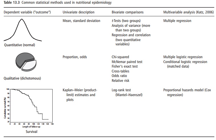
Options for statistical approaches to data analysis

Different statistical procedures are used for describing or analyzing data in nutritional epidemiology (Table 13.3). The criteria for selecting the appropriate procedure are based on the nature of the variable considered as the outcome or dependent variable. Three main types of dependent variable can be considered: quantitative (normal), qualitative (very often dichotomous), and survival or time-to-event variables.

Within bivariate comparisons, some modalities deserve further insights (Table 13.4).

The validity of most standard tests depends on the assumptions that:

●the data are from a normal distribution

●the variability within groups (if these are com-pared) is similar.

Tests of this type are termed parametric and are to some degree sensitive to violations of these assump-tions. Alternatively, nonparametric or distribution-free tests, which do not depend on the normal distribution, can be used. 

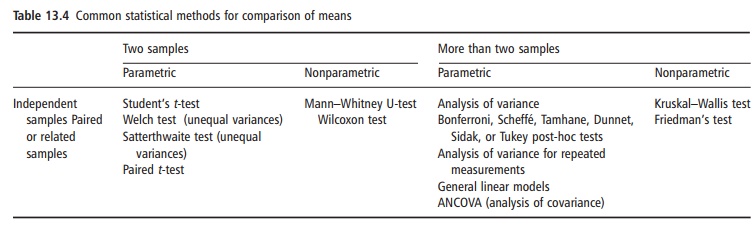
Nonparametric tests are also useful for data collected as ordinal variables because they are based on ranking the values. Relative to their parametric counterparts, nonparametric tests have the advantage of ease, but the disadvantage of less statistical power if a normal distribution should be assumed. Another additional disadvantage is that they do not permit confidence intervals for the differ-ence between means to be estimated.

A common problem in nutrition literature is mul-tiple significance testing. Some methods to consider in these instances are analysis of variance together with multiple-comparison methods specially designed to make several pairwise comparisons, such as the least significant difference method, the Bonferroni and Scheffé procedures, and the Duncan test. Analysis of variance can also be used for replicate measure-ments of a continuous variable.

Correlation is the statistical method to use when studying the association between two continuous variables. The degree of association is ordinarily mea-sured by Pearson’s correlation coefficient. This calcu-lation leads to a quantity that can take any value from −1 to +1. The correlation coefficient is positive if higher values of one variable are related to higher values of the other and it is negative when one vari-able tends to be lower while the other tends to be higher. The correlation coefficient is a measure of the scatter of the points when the two variables are plotted. The greater the spread of the points, the lower the correlation coefficient. Correlation involves an estimate of the symmetry between the two quantita-tive variables and does not attempt to describe their relationship. The nonparametric counterpart of Pearson’s correlation coefficient is the Spearman rank correlation. It is the only nonparametric method that allows confidence intervals to be estimated.

To describe the relationship between two continu-ous variables, the mathematical model most often used is the straight line. This simplest model is known as simple linear regression analysis. Regression analysis is commonly used not only to quantify the association between two variables, but also to make predictions based on the linear relationship. Nowa-days, nutritional epidemiologists frequently use the statistical methods of multivariable analysis (Table 13.3). These methods usually provide a more accurate view of the relationship between dietary and non-dietary exposures and the occurrence of a disease or other outcome, while adjusting simultaneously for many variables and smoothing out the irregularities that very small subgroups can introduce into alterna-tive adjustment procedures such as stratified analysis (Katz, 2006).

Most multivariate methods are based on the concept of simple linear regression. An explanation of the variation in a quantitative dependent variable (outcome) by several independent variables (expo-sures or predictors) is the basis of a multiple-regression model. However, in many studies the dependent variable or outcome is quite often dichoto-mous (diseased/nondiseased) instead of quantitative and can also be explained by several independent factors (dietary and nondietary exposures). In this case, the statistical multivariate method that must be applied is multiple logistic regression. In follow-up studies, the time to the occurrence of disease is also taken into account. More weight can be given to earlier cases than to later cases. The multivariate method most appropriate in this setting is the pro-portional hazards model (Cox regression) using a time-to-event variable as the outcome (Table 13.3).