Short run Cost Curves

Short run Cost Curves

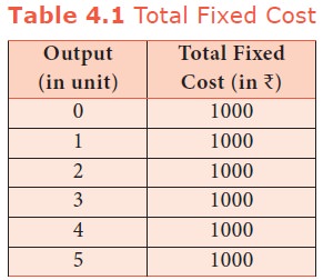
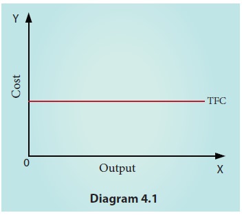
1. Total Fixed Cost (TFC)

All payments for the fixed factors of production are known as Total Fixed Cost. A hypothetical TFC is shown in table 4.1 and diagram 4.1

For instance if TC = Q3 –18Q2 + 91Q +12, the fixed cost here is 12. That means, if Q is zero, the Total cost will be 12, hence fixed cost.

It could be observed that TFC does not change with output. Even when the output is zero, the fixed cost is  Rs..1000. TFC is a horizontal straight line, parallel to X axis.

2. Total Variable Cost (TVC)

All payments to the variable factors of production is called as Total Variable Cost. Hypothetical TVC is shown in table-4.2 and Diagram 4.2

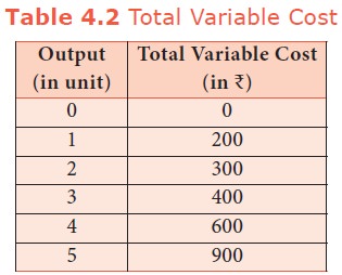
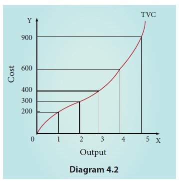
In the diagram the TVC is zero when nothing is produced. As output increases TVC also increases. TVC curve slopes upward from left to right. For instance in TC = Q³ – 18Q² + 91Q +12, variable cost, TVC = Q³ – 18Q² + 91Q

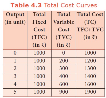
3. Total Cost Curves

Total Cost means the sum total of all payments made in the production. It is also called as Total Cost of Production. Total cost is the summation of Total Fixed Cost (TFC) and Total Variable Cost (TVC). It is written symbolically as

TC = TFC + TVC. For example, when the total fixed cost is  Rs. 1000 and the total variable cost is  Rs. 200 then the Total cost is =  Rs. 1200 ( Rs. 1000 +  Rs. 200).

If TFC = 12 and

TVC = Q³ – 18Q² + 91Q

TC = 12 + Q³ – 18Q² + 91Q

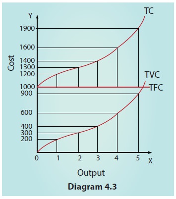
It is to be noted that

a.        The TC curve is obtained by adding TFC and TVC curves vertically.

b.        TFC curve remains parallel to x axis, indicating a straight line.

c.         TVC starts from the origin and moves upwards, as no variable cost is incurred at zero output.

d.        When TFC and TVC are added, TC starts from TFC and moves upwards.

e.         TC curve lies above the TVC curve

f.          TVC and TC curves are the same shapes but beginning point is different.

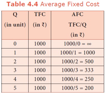
4. Average Fixed Cost (AFC)

It refers to the fixed cost per unit of output. It is obtained by dividing the total fixed cost by the quantity of output. AFC = TFC / Q where, AFC denotes average fixed cost, TFC denotes total fixed cost and Q denotes quantity of output. For example, if TFC is 1000 and the quantity of output is 10, the AFC is  Rs. 100, obtained by dividing  Rs. 1000 by 10. TVC is shown in table 4.4 and Diagram 4.4.

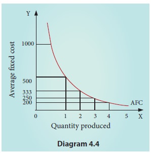
It is to be noted that

a.        AFC declines as output increases, as fixed cost remains constant

b.        AFC curve is a downward sloping throughout its length, never touching X and Y axis. It is asymptotic to both the axes.

c.         The shape of the AFC curve is a rectangular hyperbola.

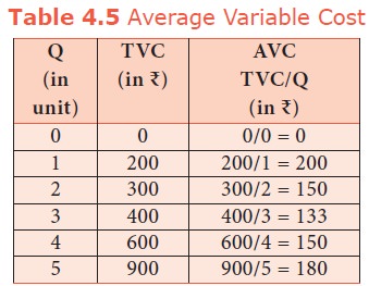
5. Average Variable Cost (AVC) 

It refers to the total variable cost per unit of output. It is obtained by dividing total variable cost (TVC) by the quantity of output (Q). AVC = TVC / Q where, AVC denotes Average Variable cost, TVC denotes total variable cost and Q denotes quantity of output. For example, When the TVC is  Rs. 300 and the quantity produced is 2, the AVC is  Rs. 150, (AVC = 300/2 = 150) AVC is shown in table 4.5 and Diagram 4.5. If TVC = Q³ – 18Q² + 91Q

AVC = Q² –18Q + 91

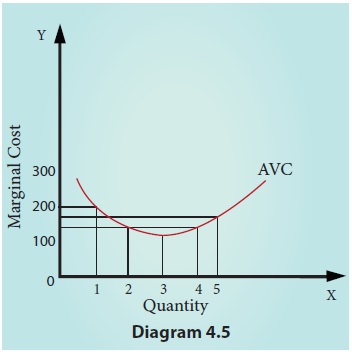
It is to be noted that

a.        AVC declines initially and then increases with the increase of output.

b.        AVC declines up to a point and moves upwards steeply, due to the law of returns.

c.         AVC curve is a U-shaped curve.

6. Average Total Cost (ATC) or Average Cost (AC)

It refers to the total cost per unit of output.

It can be obtained in two ways.

1. By dividing the firm’s total cost (TC) by the quantity of output (Q). ATC = TC / Q. For example, if TC is  Rs. 1600 and quantity of output is Q=4, the Average Total Cost is  Rs. 400.  

(ATC = 1600/4 = 400) If ATC is Q³   – 18Q² + 91Q +12, then AC = Q² – 18Q +91 12/Q

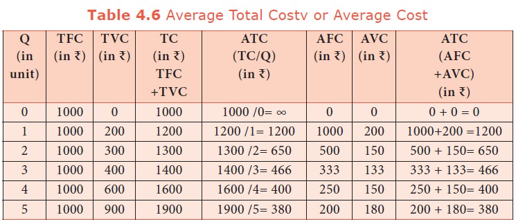
2. ByATC is derived by adding together Average Fixed Cost (AFC) and Average Variable Cost (AVC) at each level of output. ATC = AFC + AVC. For example, when Q= 2, TFC = 1000, TVC=300; AFC=500; AVC=150;ATC=650. ATC or AC is shown in table 4.6 and Diagram 4.6

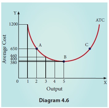
It should be noted that

a)        ATC curve is also a ‘U’ shaped curve.

b)       Initially the ATC declines, reaches a minimum when the plant is operated optimally, and rises beyond the optimum output.

c)        The ‘U’ shape of the AC reflects the law of the variable proportions.

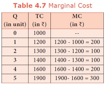
7. Marginal Cost (MC)

It is the cost of the last single unit produced. It is defined as the change in total costs resulting from producing one extra unit of output. In other words, it is the addition made to the total cost by producing one extra unit of output. 

Marginal cost is important for deciding whether any additional output can be produced or not. MC = ∆TC / ∆Q where MC denotes Marginal Cost, ∆TC denotes change in total cost and ∆Q denotes change in total quantity. For example, a firm produces 4 units of output and the Total cost is  Rs. 1600. When the firm produces one more unit (4 +1 = 5 units) of output at the total cost of  Rs. 1900, the marginal cost is  Rs. 300.

MC = 1900 – 1600 =  Rs. 300.

The other method of estimating MC is :

MC=TC_n –TC_n-1 or ^- TC_n+1 –TC_n

where, ‘MC’ denotes Marginal Cost, ‘TC_n’ denotes Total cost of ‘n’^th item, TC_n-1 denotes Total Cost of ‘n-1’ ^th item, TC_n+1 denotes Total Cost of n+1 th item. For example,

when TC4 = Rs.1600, TC(4-1)=Rs.1400 and then MC= Rs.200, (MC=1600-1400)

when TC4 = Rs.1600, TC(4+1)=1900 and then MC= 300.

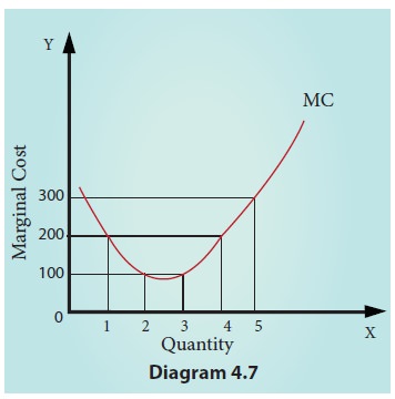
MC schedule is shown in Table 4.7 and MC Curve is shown in diagram 4.7. It is to be noted that

a)        MC falls at first due to more efficient use of variable factors.

b)       MC curve increases after the lowest point and it slopes upward.

c)        MC cure is a U-shaped curve.

d)       The slope of TC is MC.

If TC = Q³ –18Q² + 91Q +12

MC = 3Q² – 36Q +91

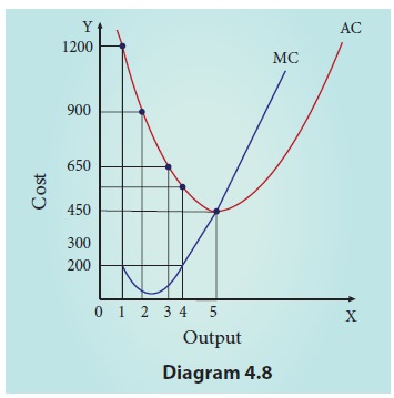
8. The relationship between Average Cost and Marginal cost

There is a unique relationship between the AC and MC curves as shown in diagram 4.8.

1.        When AC is falling, MC lies below AC.

2.        When AC becomes constant, MC also becomes equal to it.

3.        When AC starts increasing, MC lies above the AC.

4.        MC curve always cuts AC at its minimum point from below.