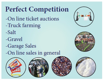
Perfect Competition

Perfect Competition:

It is an ideal but imaginary market. 100% perfect completion cannot be seen. Perfect Competition market is that type of market in which the number of buyers and sellers is very large, all are engaged in buying and selling a homogenous product at uniform price without any artificial restrictions and possessing perfect knowledge of the market at a time.

According to Joan Robinson, “Perfect competition prevails when the demand for the output of each producer is perfectly elastic”.

1. Features of the Perfect Combination:

a. Large Number of Buyers and Sellers

‘A large number of buyers’ implies that each individual buyer buys a very, very small quantum of a product as compared to that found in the market. This means that he (he includes she also) has no power to fix the price of the product. He is only a price-taker and not a price-maker.

The term, ‘large number of sellers’ implies that share of each individual seller is a very, very small quantum of a product. This means that he has no power to fix the price of the product. Like the buyer, the seller also is only a price-taker and not a price-maker.

b. Homogeneous Product and Uniform Price

The product sold and bought is homogeneous in nature, in the sense that the units of the product are perfectly substitutable. All the units of the product are identical (ie) of the same size, shape, colour, quality etc. Therefore, a uniform price prevails in the market.

c. Free Entry and Exit

In the short run, it is possible for the very efficient producer, producing the product at a very low cost, to earn super normal profits. Attracted by such a profit, new firms enter into the industry. When large number of firms enter, the supply (in comparison to demand) would increase, resulting in lower price.

An inefficient producer, who is unable to bring down the cost incurs loss. Disturbed by the loss, the existing loss-incurring firms quit the market. If it happens, supply will then decrease, price will go up. Existing firms could earn more profit.

d. Absence Of Transport Cost

The prevalence of the uniform price is also due to the absence of the transport cost.

e. Perfect Mobility of Factors of Production

The prevalence of the uniform price is also due to the perfect mobility of the factors of production. As they enjoy perfect freedom to move from one place to another and from one occupation to another, the price gets adjusted.

f. Perfect Knowledge of the Market

All buyers and sellers have a thorough knowledge of the quality of the product, prevailing price etc.

g. No Government Intervention

There is no government regulation on supply of raw materials, and in the determination of price etc.

2. Perfect Competition: Firm’s Equilibrium in the Short Run

In the short run, at least a few factors of production are fixed. The firms under Perfect Competition take the price (10) from the industry and start adjusting their quantities produced. For example Qd= 100 – 5P and Qs=5P. At equilibrium Qd=Qs. Therefore 100-5P=5P

100 = 10P; 100/10 = P

Q_d = demand

P = 10

P = Price

Qd = 100-5(10)

Q_s = Supply

100-50 = 50

Qs = 5(10)=50

Therefore 50 = 50

This diagram consists of three panels. The equilibrium of an industry is explained in the first panel. The demand and supply forces of all the firms interact and the price is fixed as Rs.10. The equilibrium of an industry is obtained at 50 units of output.

In the second part of the diagram, AC curve is lower than the price line. The equilibrium condition is achieved where MC=MR. Its equilibrium quantity sold is 50. With the prevailing price, Rs.10 it experiences super normal profit. AC = Rs.8, AR = Rs.10.

Price & Output Determination-Perfect Competition during Short Run

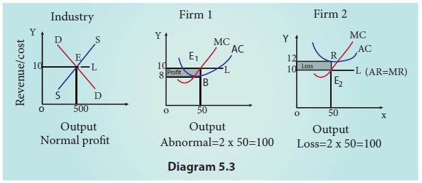
Its total revenue is 50X10=500. Its total cost is 50X8=400. Therefore, its total profit is 500-400=100.

In the third part of the diagram, firm’s cost curve is above the price line. The equilibrium condition is achieved at point where MR=MC. Its quantity sold is 50. With the prevailing price, it experiences loss. (AC>AR)

Its total revenue is 50X10=500. Its total cost is 50X12=600. Therefore, its total loss is 600-500=100.

As profit prevails in the market, new firms will enter the industry, thus increasing the supply of the product. This means a decline in the price of the product and increase the cost of production. Thus, the abnormal profit will be wiped out; loss will be incurved.

When loss prevails in the market, the existing loss making firms will exit the industry, thus decreasing the supply of the product. This means a rise in the price of the product and reduction in the cost of production. So the loss will vanish; Profit will emerge. Consequent upon the entry and exit of new firms into the industry, firms always earn ‘normal profit’ in the long run as shown in diagram.

3. Perfect Competition: Firm’s Equilibrium in the Long Run (Normal Profit)

In the long run, all the factors are variable.

The LAC curve is an envelope curve as it contains a few average cost curves. It is a flatter U shaped one. It is also known as planning curve. First, the firms will earn only normal profit.

Secondly, all the firms in the market are in equilibrium. This means that there should neither be a tendency for the new firms to enter into the industry nor for any of the existing firms to exit from the industry. 

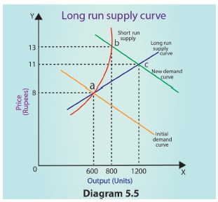
Long run supply curve is explained to determine the long run price after an increase in demand. The effect of the increase in demand in the short run is explained by the movement from point ‘a’ to point ‘b’. The price increases from  Rs.8 to  Rs.13, and the quantity increases from 600 to 800 units. Economic profit of a firm is positive. Therefore, new firms enter the market. In the long run new firms entry will continue until the price drops to  Rs.11 and the quantity is 1,200 units. The new long run equilibrium is shown by point ‘c’, where the new demand curve intersects supply curve. At this price level ( Rs.11) and quantity (1,200 units). Due to diminishing returns, it is very difficult to increase output in the short tun, as a result the price will increase to cover these higher cost of production. New firms will enter into the market. The price gradually drops to the point ( Rs.11) at which each firm makes zero economic profit.

A firm under perfect competition even in the long run is a price – taker, not a price – maker. It takes the price of the product from the industry. And it superimposes its cost curves on the revenue curves.

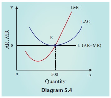
Long run equilibrium of the firm is illustrated in the diagram. Under perfect competition, long run equilibrium is only at minimum point of LAC. At point E, LMC = MR = AR = LAC.

In the above diagram (5.4), average cost is equal to average revenue. The equilibrium of the firm finally rests at point E where price is 8 and output is 500. (Numbers are hypothetical) At this point, the profit of the firm is only normal. Thus condition for long run equilibrium of the firm is:

Price = AR=MR = Minimum AC

At the equilibrium point, the SAC>LAC. Hence, long run equilibrium price is lower than short run equilibrium price; long run equilibrium quantity is larger than short run equilibrium quantity.