Chapter: Fundamentals of Database Systems : Database Design Theory and Normalization : Basics of Functional Dependencies and Normalization for Relational Databases
Normal Forms Based on Primary Keys
Normal Forms Based on Primary Keys
Having
introduced functional dependencies, we are now ready to use them to specify
some aspects of the semantics of relation schemas. We assume that a set of
functional dependencies is given for each relation, and that each relation has
a designated primary key; this information combined with the tests (conditions)
for normal forms drives the normalization
process for relational schema design. Most practical relational design
projects take one of the following two approaches:
Perform a conceptual schema design using a
conceptual model such as ER or EER and map the conceptual design into a set of
relations
Design the relations based on external knowledge
derived from an existing implementation of files or forms or reports
Following
either of these approaches, it is then useful to evaluate the relations for
goodness and decompose them further as needed to achieve higher normal forms,
using the normalization theory presented in this chapter and the next. We focus
in
this
section on the first three normal forms for relation schemas and the intuition
behind them, and discuss how they were developed historically. More general
definitions of these normal forms, which take into account all candidate keys
of a relation rather than just the primary key, are deferred to Section 15.4.
We start
by informally discussing normal forms and the motivation behind their
development, as well as reviewing some definitions from Chapter 3 that are
needed here. Then we discuss the first normal form (1NF) in Section 15.3.4, and
present the definitions of second normal form (2NF) and third normal form
(3NF), which are based on primary keys, in Sections 15.3.5 and 15.3.6,
respectively.
1. Normalization of
Relations
The normalization process, as first proposed by Codd (1972a), takes a
relation schema through a series of tests to certify whether it satisfies a certain normal form. The process, which proceeds in a top-down fashion by
evaluating each relation against the criteria for normal forms and decomposing
relations as necessary, can thus be considered as relational design by analysis. Initially, Codd proposed three
normal forms, which he called first, second, and third normal form. A stronger
definition of 3NF—called Boyce-Codd normal form (BCNF)—was proposed later by
Boyce and Codd. All these normal forms are based on a single analytical tool:
the functional dependencies among the attributes of a relation. Later, a fourth
normal form (4NF) and a fifth normal form (5NF) were proposed, based on the
concepts of multivalued dependencies and join dependencies, respectively; these
are briefly dis-cussed in Sections 15.6 and 15.7.
Normalization of data can be considered a process of analyzing the given relation schemas based on their FDs and primary
keys to achieve the desirable properties of
(1) minimizing redundancy and (2) minimizing the insertion, deletion,
and update anomalies discussed in Section 15.1.2. It can be considered as a
“filtering” or “purification” process to make the design have successively
better quality. Unsatisfactory relation schemas that do not meet certain
conditions—the normal form tests—are
decomposed into smaller relation schemas that meet the tests and hence possess
the desirable properties. Thus, the normalization procedure provides database
designers with the following:
A formal framework for analyzing
relation schemas based on their keys and on the functional dependencies among
their attributes
A series of normal form tests
that can be carried out on individual relation schemas so that the relational
database can be normalized to any
desired degree
Definition. The normal form of a relation
refers to the highest normal form condition
that it meets, and hence indicates the degree to which it has been normalized.
Normal forms, when considered in
isolation from other factors, do not guarantee a good database design. It
is generally not sufficient to check separately that each relation schema in
the database is, say, in BCNF or 3NF. Rather, the process of normalization
through decomposition must also confirm the existence of additional properties
that the relational schemas, taken together, should possess. These would
include two properties:
The nonadditive join or lossless join property, which guarantees that
the spurious tuple generation problem discussed in Section 15.1.4 does not
occur with respect to the relation schemas created after decomposition.
The dependency preservation property, which ensures that each
functional dependency is represented in some individual relation resulting
after decomposition.
The nonadditive join property is extremely critical and must be achieved at any cost, whereas the dependency
preservation property, although desirable, is some-times sacrificed, as we
discuss in Section 16.1.2. We defer the presentation of the for-mal concepts
and techniques that guarantee the above two properties to Chapter 16.
2. Practical Use of
Normal Forms
Most practical design projects acquire existing designs of databases
from previous designs, designs in legacy models, or from existing files.
Normalization is carried out in practice so that the resulting designs are of
high quality and meet the desirable properties stated previously. Although
several higher normal forms have been defined, such as the 4NF and 5NF that we
discuss in Sections 15.6 and 15.7, the practical utility of these normal forms becomes
questionable when the constraints on which they are based are rare, and hard to
understand or to detect by the data-base designers and users who must discover
these constraints. Thus, database design as practiced in industry today pays
particular attention to normalization only up to 3NF, BCNF, or at most 4NF.
Another point worth noting is that the database designers need not normalize to the highest
possible normal form. Relations may be left in a lower normalization status,
such as 2NF, for performance reasons, such as those discussed at the end of
Section 15.1.2. Doing so incurs the corresponding penalties of dealing with the
anomalies.
Definition. Denormalization is the process of storing the join of higher nor-mal form relations as a
base relation, which is in a lower normal form.
3. Definitions of Keys and
Attributes Participating in Keys
Before
proceeding further, let’s look again at the definitions of keys of a relation
schema from Chapter 3.
Definition. A superkey of a relation schema
R = {A1, A2,
... , An} is a set of attributes
S ⊆ R with the property that no two tuples t1 and t2 in any legal rela-tion state r of R will have t1[S] = t2[S]. A key K is a superkey with
the additional property that removal of any attribute from K will cause K not to be
a superkey any more.
The
difference between a key and a superkey is that a key has to be minimal; that is,
if we
have a key K = {A1, A2,
..., Ak} of R, then K – {Ai} is
not a key of R for any Ai, 1 ≤ i ≤ k. In
Figure 15.1, {Ssn} is a
key for EMPLOYEE, whereas {Ssn}, {Ssn, Ename},
{Ssn, Ename, Bdate}, and
any set of attributes that includes Ssn are all
superkeys.
If a
relation schema has more than one key, each is called a candidate key. One of the candidate keys is arbitrarily designated to be the primary key, and the others are called secondary keys. In a
practical relational database, each relation schema must have a primary key. If
no candidate key is known for a relation, the entire relation can be treated as
a default superkey. In Figure 15.1, {Ssn} is the
only candidate key for EMPLOYEE, so it
is also the primary key.
Definition. An attribute of relation schema R is called a prime attribute of R
if it is a member of some candidate key of R. An attribute is called nonprime if it is not a prime
attribute—that is, if it is not a member of any candidate key.
In Figure
15.1, both Ssn and Pnumber are prime attributes of WORKS_ON, whereas other attributes of WORKS_ON are nonprime.
We now
present the first three normal forms: 1NF, 2NF, and 3NF. These were pro-posed
by Codd (1972a) as a sequence to achieve the desirable state of 3NF relations
by progressing through the intermediate states of 1NF and 2NF if needed. As we
shall see, 2NF and 3NF attack different problems. However, for historical
reasons, it is customary to follow them in that sequence; hence, by definition
a 3NF relation already satisfies 2NF.
4. First Normal Form
First normal form (1NF) is now
considered to be part of the formal definition of a relation in the basic (flat) relational model; historically, it
was defined to disallow multivalued attributes, composite attributes, and their
combinations. It states that the domain of an attribute must include only atomic (simple, indivisible) values and that the value of any
attribute in a tuple must be a single
value from the domain of that attribute. Hence, 1NF disallows having a set
of values, a tuple of values, or a combination of both as an attribute value
for a single tuple. In other words,
1NF dis-allows relations within relations
or relations as attribute values within
tuples. The only attribute values permitted by 1NF are single atomic (or indivisible) values.
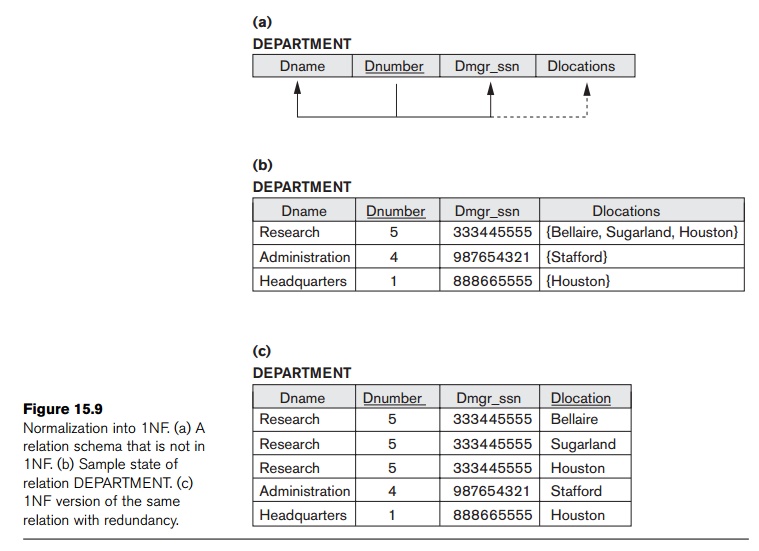
Consider
the DEPARTMENT relation schema shown in Figure
15.1, whose primary key is Dnumber, and
suppose that we extend it by including the Dlocations
attribute as shown in Figure 15.9(a). We assume that each department can have a number of locations. The DEPARTMENT schema and a sample relation
state are shown in Figure 15.9. As we can see, this is not in 1NF because Dlocations is not an atomic attribute, as
illustrated by the first tuple in Figure 15.9(b). There are two ways we can
look at the Dlocations
attribute:
The
domain of Dlocations contains
atomic values, but some tuples can have a set of these values. In this case, Dlocations is not functionally dependent on the primary key Dnumber.
The domain of Dlocations contains sets of values and hence is nonatomic. In this case, Dnumber → Dlocations because each set is considered a single member of the attribute domain.
In either
case, the DEPARTMENT relation
in Figure 15.9 is not in 1NF; in fact, it does not even qualify as a relation
according to our definition of relation in Section 3.1. There are three main
techniques to achieve first normal form for such a relation:
1.
Remove the attribute Dlocations that violates 1NF and
place it in a separate relation DEPT_LOCATIONS along with the primary key Dnumber of DEPARTMENT. The primary key of this relation is
the combination
Dnumber, Dlocation}, as shown in Figure 15.2. A distinct tuple in DEPT_LOCATIONS exists for each location of a department. This
decomposes the non-1NF relation into two 1NF relations.
Expand the key so that there will be a separate
tuple in the original DEPARTMENT relation
for each location of a DEPARTMENT, as
shown in Figure 15.9(c). In this case, the
primary key becomes the combination {Dnumber, Dlocation}. This solution has the
disadvantage of introducing redundancy in
the relation.
If a maximum number of values is known for the attribute—for example, if it is known that at most three locations can exist for a department—replace the Dlocations attribute by three atomic attributes: Dlocation1, Dlocation2, and Dlocation3. This solution has the disadvantage of introducing NULL values if most departments have fewer than three locations. It further introduces spurious semantics about the ordering among the location values that is not originally intended. Querying on this attribute becomes more difficult; for example, consider how you would write the query: List the departments that have ‘Bellaire’ as one of their locations in this design.
Of the
three solutions above, the first is generally considered best because it does
not suffer from redundancy and it is completely general, having no limit placed
on a maximum number of values. In fact, if we choose the second solution, it
will be decomposed further during subsequent normalization steps into the first
solution.
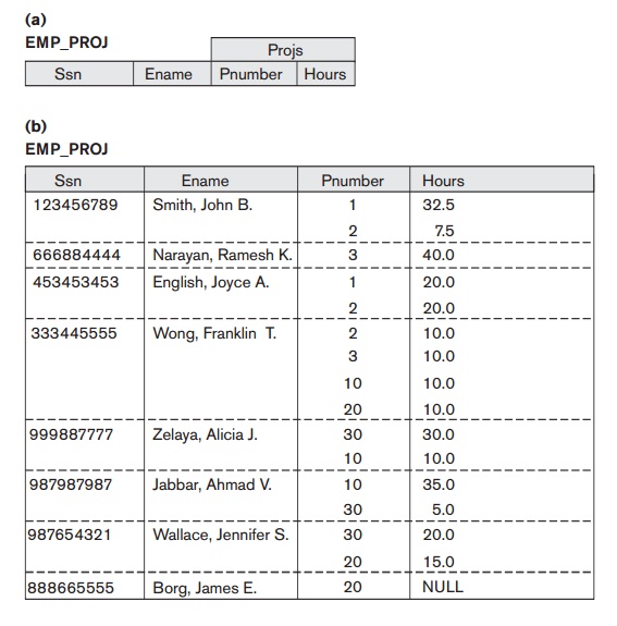
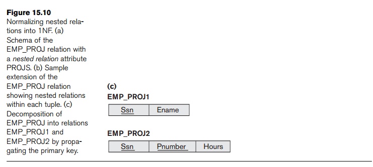
First
normal form also disallows multivalued attributes that are themselves
composite. These are called nested
relations because each tuple can have a relation within it. Figure 15.10 shows how the EMP_PROJ relation could appear if nesting
is allowed. Each tuple represents an
employee entity, and a relation PROJS(Pnumber, Hours) within each tuple represents the employee’s
projects and the hours per week that
employee works on each project. The schema of this EMP_PROJ relation can be represented as
follows:
EMP_PROJ(Ssn, Ename, {PROJS(Pnumber, Hours)})
The set
braces { } identify the attribute PROJS as
multivalued, and we list the component attributes that form PROJS between parentheses ( ).
Interestingly, recent trends for supporting complex objects (see Chapter 11)
and XML data (see Chapter 12) attempt to allow and formalize nested relations
within relational database systems, which were disallowed early on by 1NF.
Notice
that Ssn is the primary key of the EMP_PROJ relation in Figures 15.10(a) and
(b), while Pnumber is the partial key of the nested relation;
that is, within each tuple, the nested relation must have unique values of Pnumber. To normalize this into 1NF, we
remove the nested relation attributes into a new relation and propagate the primary key into it; the
primary key of the new relation will combine the partial key with the primary key of the original
relation. Decomposition and primary key propagation yield the schemas EMP_PROJ1 and EMP_PROJ2, as shown in Figure 15.10(c).
This
procedure can be applied recursively to a relation with multiple-level nesting
to unnest the relation into a set of
1NF relations. This is useful in converting an unnormalized relation schema
with many levels of nesting into 1NF relations. The
existence
of more than one multivalued attribute in one relation must be handled
carefully. As an example, consider the following non-1NF relation:
PERSON (Ss#, {Car_lic#}, {Phone#})
This
relation represents the fact that a person has multiple cars and multiple
phones. If strategy 2 above is followed, it results in an all-key relation:
PERSON_IN_1NF (Ss#, Car_lic#, Phone#)
To avoid
introducing any extraneous relationship between Car_lic# and Phone#, all
possible combinations of values are represented for every Ss#, giving rise to redundancy.
This leads to the problems handled by multivalued dependencies and 4NF, which
we will discuss in Section 15.6. The right way to deal with the two
multivalued attributes in PERSON shown
previously is to decompose it into two separate relations, using strategy 1
discussed above: P1(Ss#, Car_lic#) and P2(Ss#, Phone#).
5. Second Normal Form
Second normal form (2NF) is based
on the concept of full functional dependency. A
functional dependency X → Y is a full functional
dependency if removal of any attribute A
from X means that the dependency does
not hold any more; that is, for any attribute A ε X, (X
– {A}) does not functionally determine Y.
A functional dependency X → Y is a partial dependency
if some attribute A ε X can be removed from X
and the dependency still holds; that is, for some A ε X, (X
– {A}) → Y. In Figure 15.3(b), {Ssn, Pnumber} → Hours is a full dependency (neither Ssn → Hours nor Pnumber → Hours holds). However, the dependency
{Ssn, Pnumber} → Ename is partial because Ssn → Ename holds.
Definition. A relation schema R is in 2NF if every nonprime attribute A in
R is fully functionally dependent on the primary key of R.
The test
for 2NF involves testing for functional dependencies whose left-hand side
attributes are part of the primary key. If the primary key contains a single
attribute, the test need not be applied at all. The EMP_PROJ relation in Figure 15.3(b) is in
1NF but is not in 2NF. The nonprime attribute Ename violates 2NF because of FD2, as do
the nonprime attributes Pname and Plocation because of FD3. The functional dependencies FD2 and FD3 make Ename, Pname, and Plocation
partially dependent on the primary key {Ssn, Pnumber} of EMP_PROJ, thus violating the 2NF test.
If a
relation schema is not in 2NF, it can be second
normalized or 2NF normalized into
a number of 2NF relations in which nonprime attributes are associated only with
the part of the primary key on which they are fully functionally dependent.
Therefore, the functional dependencies FD1, FD2, and FD3 in Figure 15.3(b) lead to the
decomposition of EMP_PROJ into the
three relation schemas EP1, EP2, and EP3 shown in Figure 15.11(a), each
of which is in 2NF.
6. Third Normal Form
Third normal form (3NF) is based
on the concept of transitive dependency. A functional dependency X → Y in a relation schema R is a transitive dependency if there exists a set of attributes Z in R
that is neither a candidate key nor a subset of any key of R,10 and both X
→ Z and Z → Y hold. The dependency Ssn → Dmgr_ssn is transitive through Dnumber in EMP_DEPT in Figure 15.3(a), because both
the dependencies Ssn → Dnumber and Dnumber → Dmgr_ssn hold and
Dnumber is nei-ther a key itself nor a
subset of the key of EMP_DEPT.
Intuitively, we can see that the dependency of
Dmgr_ssn on Dnumber is undesirable in since Dnumber
is not a
key of EMP_DEPT.
Definition. According to Codd’s original
definition, a relation schema R
is in 3NF if it satisfies 2NF and no nonprime attribute of R is transitively dependent on the primary key.
The
relation schema EMP_DEPT in
Figure 15.3(a) is in 2NF, since no partial depen-dencies on a key exist.
However, EMP_DEPT is not
in 3NF because of the transitive dependency of Dmgr_ssn (and also Dname) on Ssn via Dnumber. We can normalize EMP_DEPT by decomposing it into the two
3NF relation schemas ED1 and ED2 shown in Figure 15.11(b).
Intuitively, we see that ED1 and ED2 represent independent entity
facts about employees and departments. A NATURAL
JOIN
operation on ED1 and ED2 will recover the original
relation EMP_DEPT without generating spurious
tuples.
Intuitively,
we can see that any functional dependency in which the left-hand side is part
(a proper subset) of the primary key, or any functional dependency in which the
left-hand side is a nonkey attribute, is a problematic
FD. 2NF and 3NF normalization remove these problem FDs by decomposing the
original relation into new relations. In terms of the normalization process, it
is not necessary to remove the partial dependencies before the transitive
dependencies, but historically, 3NF has been defined with the assumption that a
relation is tested for 2NF first before it is tested for 3NF. Table 15.1
informally summarizes the three normal forms based on primary keys, the tests
used in each case, and the corresponding remedy
or normalization performed to achieve the normal form.
Related Topics