Microsoft Office - MS Excel Practical - Computerised Accounting

MS-Excel

i) Functions

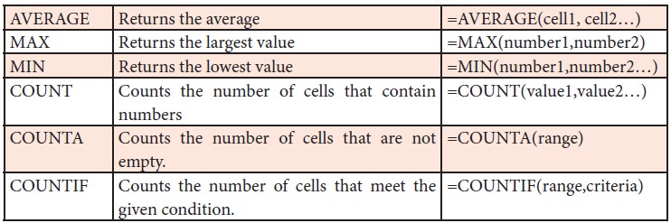
a. Statistical functions

There are several statistical functions such that are inbuilt in MS Excel. The following are explained.

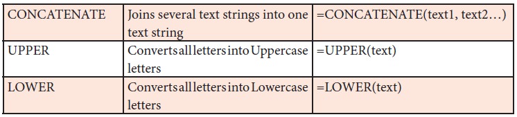
b. Text functions

There are several text functions such that are inbuilt in MS Excel. The following are explained.

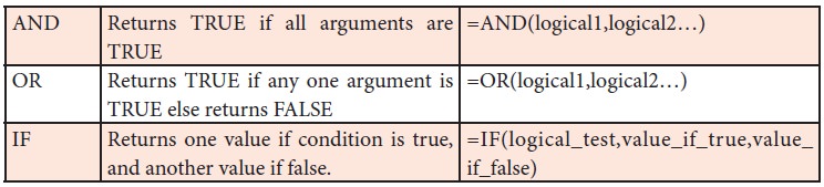
c. Logical functions

There are several logical functions such that are inbuilt in MS Excel. The following are explained.

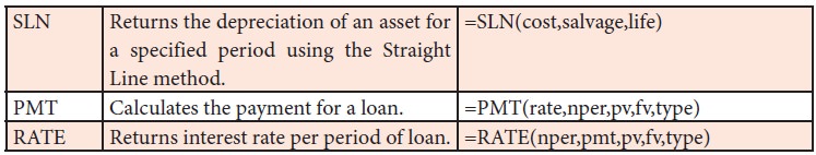
d. Financial functions

There are several financial functions such that are inbuilt in MS Excel. The following are explained.

 

MS-Excel practical

 

Illustration 3

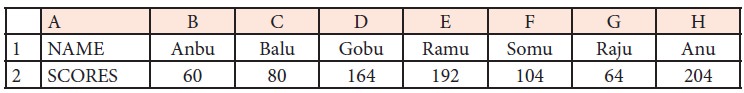
The following are the scores obtained by some students in a competitive examination. Find out the average, the highest and the lowest score using appropriate function in spreadsheet.

Solution

Procedure

i.               Open a new spreadsheet in MS-Excel

ii.               Enter all given values as given in the question.

iii.               To find the Average mark in cell B5 give the formula =AVERAGE(B2:H2)

iv.               To calculate the highest score, in cell B3 give the formula =MAX(B2:H2)

v.               To find the lowest rank in cell B4 give the formula =MIN(B2:H2)

Answer:

The average score is 124, the highest score is 204 and the lowest score is 60.

 

Illustration 4

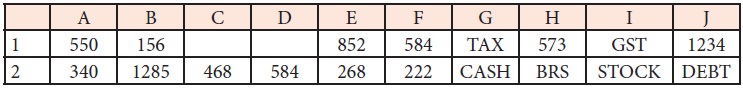
The following table is given to you. Find solution for the following questions.

A.      How many cells contain numbers only?

 

B.      Count the number of cells that contain any value.

 

C.      Count the number of cells containing the value exceeding 1000.

 

Solution

Procedure

i.               Open a new spread sheet in MS-Excel.

ii.               Enter the data in cells from A1 to J2 as in the question

iii.               To get the Number of cells containing numbers only, write the formula in B3 =COUNT(A1:J2)

iv.               To get Number of cells that contain any value, write the formula in B4 =COUNTA(A1:J2)

v.               To get the Number of cells which have values exceeding 1000, write the formula in B5=COUNTIF(A1:J2,”>1000”)

Answer

A) 12 B) 18 C) 2   b) Text functions

Illustration 5 (CONCATENATE)

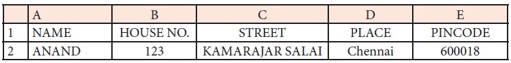
From the data given below

Fill the address in B3 using CONCATENATE Function.

 

Change KAMARAJAR SALAI given in C2 as lower case in C3

 

Change Chennai given in D2 as upper case in D3

 

Solution

Procedure

i. To fill the address

a.        Open a new spreadsheet in MS-Excel

b.        Enter all given values as given in the question

c.         Enter the formula in the cell B3 as =CONCATENATE(A2,” “,B2,” “,C2,” “,D2,” “,E2)

Answer

ANAND 123 KAMARAJAR SALAI Chennai 600018

ii. To change KAMARAJAR SALAI given in C2 as lower case in C3 Enter the formula in the cell C3 as=LOWER(C2)

Answer

kamarajar salai

iii. To change Chennai given in D2 as upper case in D3 Enter the formula in the cell D3 as=UPPER(D2)

Answer

CHENNAI

 

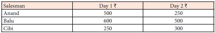
Illustration 6 (AND function)

There are three salesmen. Two days of sales achievement is given. You are required to find out the salesmen who have achieved a minimum sale of Rs.  400 on each day.

Solution

Procedure

i.               Open new excel sheet.

ii.               Input the table as given in the question.

iii.               Enter the data “Achieved” in Cell D1.

iv.               Type the following in Cell D2: =AND(B2>=400,C2>=400)

v.               Copy the formula in D2 into D3 and D4

Output

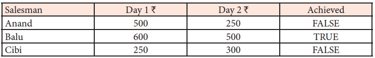
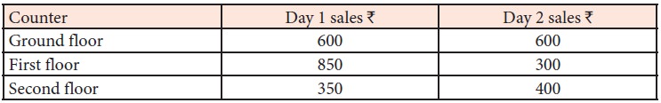
Illustration 7 (OR function)

Find out from the following data, minimum collection of Rs.  500 on any one day achieved by the sales counters.

Solution

Procedure

i.               Open new excel sheet.

ii.               Input the table as given in the question.

iii.               Enter the data “Achieved” in Cell D1.

iv.               Type the following in Cell D2: =OR(B2>=500,C2>=500)

v.               Copy the formula from D2 into D3 and D4

Output

 

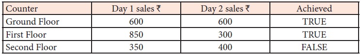
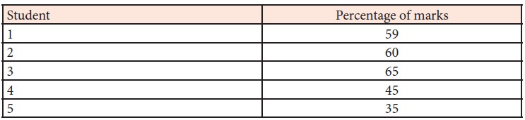
Illustration 8 (IF function)

Following is the list of students and percentage of marks obtained by them. If a student has secured a minimum of 50%, he is declared pass, else fail.

Solution

Procedure

i.               Open new excel sheet.

ii.               Input the table as given in the question.

iii.               Enter the data “Result” in Cell A3.

iv.               Type the following in Cell B3 B3=IF(B1>=50,”Pass”,”Fail”)

v.               Copy the formula from B3 to C3, D3 and E3

Output

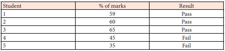
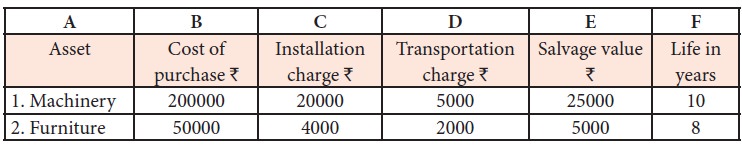
Illustration 9 (Depreciation – SLN method)

Calculate depreciation under Straight Line Method using Spreadsheet based on the details given below.

Solution

Procedure and answer

i.               Open a new spreadsheet in MS-EXCEL

ii.               Enter labels and values in the cells as given above

iii.               Write total cost in G1 and annual depreciation in H1

iv.               Calculate total cost in the cell G2 by the formula =Sum(B2:D2) and copy formula to cell G3

v.               Calculate annual depreciation in the cell H2 by the formula=SLN(G2,E2,F2) and copy formula to cell H3

Output

 

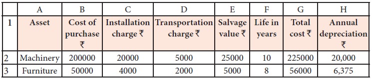
Illustration 10 (PMT)

Consider the following information:

Loan amount Rs.  3,00,000

Number of payment periods 48 months

Annual rate of interest 10%

Calculate periodic payment using PMT function.

Solution

Procedure

i.               Open a new spreadsheet in MS-Excel

ii.               Enter values in the cells as given below

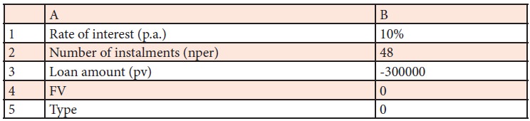
Compute PMT in the cell B6 by the formula=PMT(B1/12,B2,B3,B4,B5)

Answer Rs.  7,608.78

 

Illustration 11 (RATE)

Mr. Vivek took a loan of Rs.  2,00,000 from State Bank of India, Chennai and number of installments is 84 months. Calculate the rate assuming payments Rs.  3,300 per month using appropriate function.

Solution

Procedure

i.               Open a new spreadsheet in MS-Excel

ii.               Enter values in the cells as given below

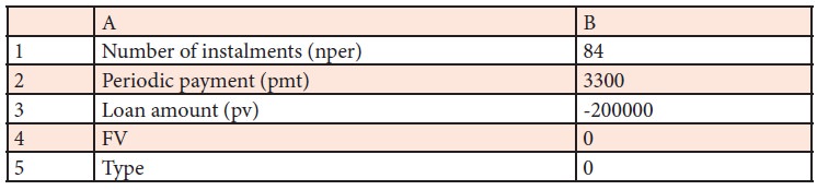
iii. Compute RATE in the cell B6 by the formula=RATE(B1,B2,B3,B4,B5)*12

Answer 10%

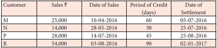
Illustration 12 (Computation of interest on overdue)

Sara Ltd., sells goods on credit basis. Their policy is to charge interest @ 2% p.a., for the period of default. From the following data, find out the amount to be collected from each customer. Assume 365 days in the year.

Solution

Procedure

i.               Open a new spreadsheet in MS-Excel

ii.               Enter the table headings as given below in different cells

A1 Customer

B1 Sales (Rs. )

C1 Date of sales

D1 Period of credit (days)

E1  Date of settlement

F1  Credit period availed (days)

G1 Days of default

H1 Interest

I1   Amount collected

iii.  Enter customer names in A2:A5

iv.  Enter sales figures in B2:B5

v.   Enter date of sales in C2:C5

vi.  Enter period of credits in D2:D5

vii. Enter date of settlements in E2:E5

viii.    In the cell F2 enter the formula =E2-C2 to calculate the period of credit availed in days.

ix.  In the cell G2 enter the formula=IF(F2-D2>0,F2-D2,0) to calculate the default days. (IF condition is used to avoid negative values in the case of payment before due date)

x.   In the cell H2 enter the formula =ROUNDUP((B2*2%)*(G2/365),0) to calculate interest for the default days and to round it to the nearest rupee.

xi.  In the cell I2 enter the formula =B2+H2 to add the amount of Sales and Interest.

xii. Select the range F2:I2 and copy these cells down to the last customer.

Output

 

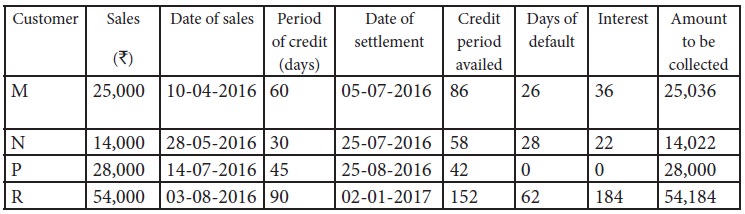
Illustration 13 (Payroll preparation)

Prepare payroll of the following employees.

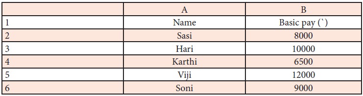
Additional information:

a. DA: 125% of basic pay

b. HRA: Rs.  4,000 for employees basic pay greater than Rs.  8,000, for others Rs.  2,500.

c. PF Contribution: 12% of basic pay and DA

d. TDS: 10% for Gross pay greater than Rs.  25,000, otherwise NIL.

Procedure

i.               Open a new spreadsheet in MS-EXCEL

ii.               Enter labels and values in the cells as given above

iii.               To calculate DA in Cell C =B2*125%

iv.               To calculate HRA in Cell D2 = IF(B2>8000,4000,2500)

v.               To calculate Gross Pay in Cell E2 =SUM(B2:D2)

vi.               To calculate PF in Cell F2 =(B2+C2)*12%

vii.               To calculate TDS in Cell G2 =IF(E2>25000,E2*10%,0)

viii.               To calculate Net Pay in Cell H2=E2-(F2+G2)

Output

 

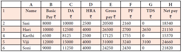
Illustration 14 (Column chart and Line chart)

The total sales volume (Product wise) of TECH Ltd for the year 2016-2017 is given below:

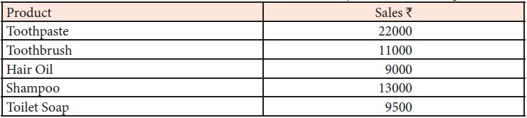
i.               Present the data in a column chart

ii.               Change the chart type to line chart.

Procedure

Column chart

i.               Enter the data given in the table in a new spreadsheet.

ii.               Select the data range from A1 to B7.

iii.               Go to Insert menu and select Column Chart (3D)

iv.               Right click column chart and select ‘Add Data Labels’

v.               Choose layout tab under Chart tools.

vi.               Select Axis title and name them.

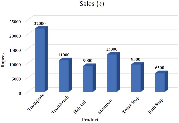
Line Chart

i.               Select the data range from A1 to B7.

ii.               Go to Insert menu and select Line Chart (2D)

iii.               Right click chart and select ‘Add Data Labels’

iv.               Choose layout tab under Chart tools.

v.               Select Axis title and name them.

 

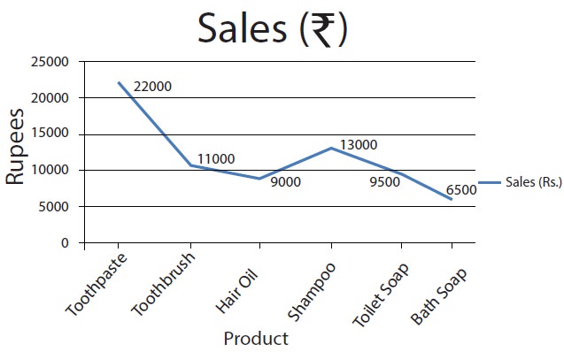
Illustration 15 (Pie Chart and Doughnut)

Sales volume of Moon Ltd during 2017 is given below.

Draw

a. Pie chart

b. Doughnut

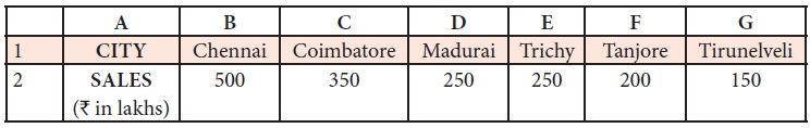
Procedure

(a) Pie chart

       i.   Enter the data given in the table in a new spreadsheet.

     ii.   Select the data range from A1 to G2.

  iii.   Go to Insert menu and select Pie Chart (3D Type)

  iv.   Right click pie chart and select ‘Add Data Labels’

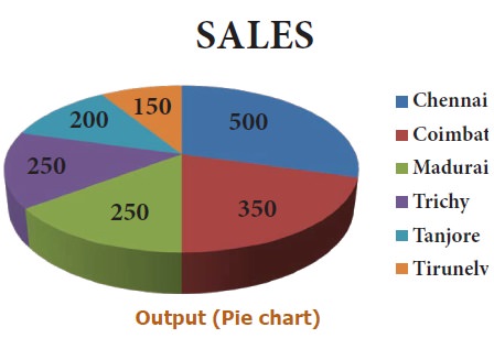
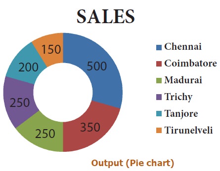
(b) Doughnut

i.               Go to Insert menu -> Other Charts and select Doughnut

ii.               Right click doughnut chart and select ‘Add Data Labels’