Marginal Productivity Theory of Distribution

Marginal Productivity Theory of Distribution

Introduction

Marginal Productivity Theory of distribution was developed by Clark, Wickseed and Walras. This theory explains how the prices of various factors of production are determined. This theory explains how rent, wages, interest and profit are determined. This theory is also known as “General Theory of Distribution” or “National Dividend Theory of Distribution”.

Assumptions

This theory is based on the following assumptions:

1.        All the factors of production are homogenous.

2.        Factors of production can be substituted for each other.

3.        There is perfect competition both in the factor market and product market.

4.        There is perfect mobility of factors of production.

5.        There is full employment of factors.

6.        This theory is applicable only in the long-run.

7.        The entrepreneurs aim at profit maximization.

8.        There is no government intervention in fixing the price of a factor.

9.        There is no technological change.

Explanation of the Theory

According to the Marginal Productivity Theory of Distribution, the price or the reward for any factor of production is equal to the marginal productivity of that factor. In short, each factor is rewarded according to its marginal productivity.

Marginal Product

The Marginal product of a factor of production means the addition made to the total product by employment of an additional unit of that factor. The Marginal Product may be expressed as MPP, VMP and MRP.

1. Marginal Physical Product (MPP)

The Marginal Physical Product of a factor is the increment in the total product obtained by the employment of an additional unit of that factor.

2. Value of Marginal Product (VMP)

The Value of Marginal Product is obtained by multiplying the Marginal Physical Product of the factor by the price of product.

Symbolically

VMP = MPP x Price

3. Marginal Revenue Product (MRP)

The Marginal Revenue Product of a factor is the increment in the total revenue which is obtained by the employment of an additional unit of that factor.

MRP = MPP x MR

Statement of the Theory

An employer employs a factor of production because it is productive. So, the price he wants to pay for the factor depends upon its productivity. The greater the productivity of a factor, the higher will be its reward. If the price of a factor of production is less

than its marginal revenue product, the employer will use more of this factor, because his profit will be increased.

When more of a factor is employed, its marginal revenue product diminishes. But the employer will gain by using additional units of the factor until the marginal revenue product of the factor is equal to its price. The employer’s profit will be maximum at this point. Beyond the point, the marginal revenue product is less than the price of the factor. Hence, employer will suffer loss when he uses more of the factor. Therefore, the conclusion is that the employer will so adjust the price of the factor of production so as to equalize the marginal revenue product of that factor.

In short, the Marginal Productivity Theory of Distribution states that

a.        The price of a factor of production depends upon its productivity.

b.        The price of a factor is determined by and will be equal to marginal revenue product of that factor.

c.         Under certain conditions, the price of a factor will be equal to both the average and marginal products of that factor.

The Marginal Productivity  Theory of Distribution can be represented

diagrammatically as follows:

Marginal Productivity under Perfect Competition

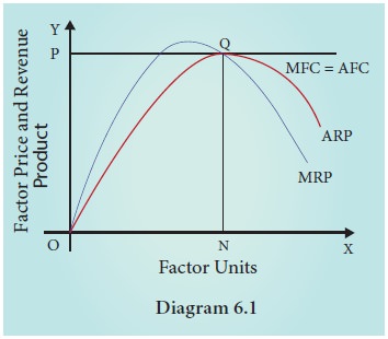
The diagram 6.1 refers to the factor pricing under perfect competition in the factor market. X axis represents factor units and Y axis represents the factor price and revenue product. MRP is the Marginal Revenue Product Curve and ARP is the Average Revenue Product curve. AFC is the Average Factor Cost curve and MFC is the Marginal Factor Cost curve. AFC is horizontal under perfect competition and MFC coincides with it.

When there is perfect competition in the factor market, the firm is in equilibrium (i.e., earning maximum profits) only when MFC = MRP. Hence, in the diagram, the firm reaches equilibrium at point Q by employing ON units of factors and paying OP price (NQ) where MFC = MRP. At the point Q, MRP = ARP. The price paid to the factor (NQ) is also equal to marginal revenue product (NQ) and average revenue product (NQ). This means that there is no exploitation of factors under perfect competition. Beyond the point Q, no employer will employ factors, because after that point, the price paid to the factor is more than marginal revenue product and average revenue product.

Marginal Productivity Theory under Imperfect Competition

In diagram 6.2 the factor pricing under imperfect competition is represented. AFC is Average Factor Cost curve. It represents the price paid to the factors. It increases as the number of factors demanded by the employer increases. As AFC rises, MFC lies above AFC. It represents the marginal cost paid to the factors. At the point Q, MFC = MRP, where the employer attains his maximum profit and so he stops employment of the factors

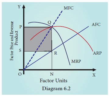
at the point. But the average cost paid is NRSO and the average revenue obtained is NQ or OP. Total revenue obtained is NQPO. Therefore, exploitation per unit of factor is RQ. But the total number of factors is ON. Thus, the total exploitation of factor by the employer is RQ X SR = “PQRS” (shaded area). Thus, under imperfect competition, factor is exploited at the equilibrium position.

Criticisms

This theory is subject to a few criticisms

a.        In reality, the factors of production are not homogenous.

b.        In practice, factors cannot be substituted for each other.

c.         This theory is applicable only in the long–run. It cannot be applied in the short-run.