Essential of Traditional Routing Protocols

ESSENTIAL OF TRADITIONAL ROUTING PROTOCOLS

Link State Routing Protocol

Link state routing has a different philosophy from that of distance vector routing. In link state routing, if each node in the domain has the entire topology of the domain the list of nodes and links, how they are connected including the type, cost (metric), and condition of the links (up or down)-the node can use Dijkstra's algorithm to build a routing table.

Concept of link state routing

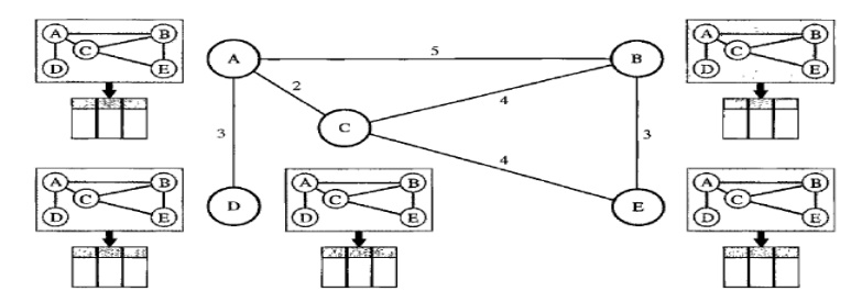
The figure shows a simple domain with five nodes. Each node uses the same topology to create a routing table, but the routing table for each node is unique because the calculations are based on different interpretations of the topology. This is analogous to a city map. While each person may have the same map, each needs to take a different route to reach her specific destination.

The topology must be dynamic, representing the latest state of each node and each link. If there are changes in any point in the network (a link is down, for example), the topology must be updated for each node.

Building Routing Tables

In link state routing, four sets of actions are required to ensure that each node has the routing table showing the least-cost node to every other node.

1. Creation of the states of the links by each node, called the link state packet (LSP).

2.  Dissemination of LSPs to every other router, called flooding, in an efficient and reliable way.

3. Formation of a shortest path tree for each node.

4. Calculation of a routing table based on the shortest path tree.

Creation of Link State Packet (LSP)

A link state packet can carry a large amount of information. For the moment, however, we assume that it carries a minimum amount of data: the node identity, the list of links, a sequence number, and age. The first two, node identity and the list of links, are needed to make the topology. The third, sequence number, facilitates flooding and distinguishes new LSPs from old ones. The fourth, age, prevents old LSPs from remaining in the domain for a long time. LSPs are generated on two occasions:

1. When there is a change in the topology of the domain. Triggering of LSP dissemination is the main way of quickly informing any node in the domain to update its topology.

2.  On a periodic basis. The period in this case is much longer compared to distance vector routing. As a matter of fact, there is no actual need for this type of LSP dissemination.

It is done to ensure that old information is removed from the domain. The timer set for periodic dissemination is normally in the range of 60 min or 2 h based on the implementation. A longer period ensures that flooding does not create too much traffic on the network.

Flooding of LSPs After a node has prepared an LSP, it must be disseminated to all other nodes, not only to its neighbours. The process is called flooding and based on the following:

1. The creating node sends a copy of the LSP out of each interface.

2.  A node that receives an LSP compares it with the copy it may already have. If the newly arrived LSP is older than the one it has (found by checking the sequence number), it discards the LSP. If it is newer, the node does the following:

a. It discards the old LSP and keeps the new one.

b. It sends a copy of it out of each interface except the one from which the packet arrived. This guarantees that flooding stops somewhere in the domain (where a node has only one interface).

Formation of Shortest Path Tree

Dijkstra Algorithm After receiving all LSPs, each node will have a copy of the whole topology. However, the topology is not sufficient to find the shortest path to every other node; a shortest path tree is needed.

A tree is a graph of nodes and links; one node is called the root. All other nodes can be reached from the root through only one single route. A shortest path tree is a tree in which the path between the root and every other node is the shortest. What we need for each node is a shortest path tree with that node as the root.

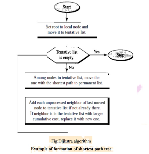
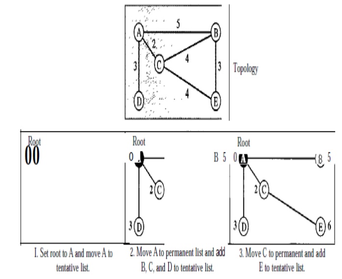
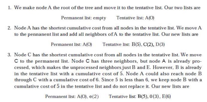
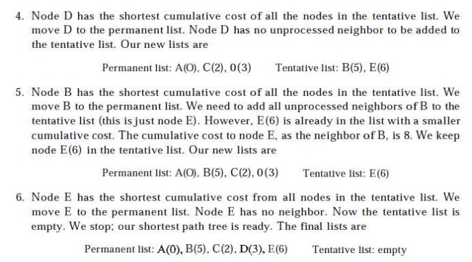
The Dijkstra algorithm creates a shortest path tree from a graph. The algorithm divides the nodes into two sets: tentative and permanent. It finds the neighbours of a current node, makes them tentative, examines them, and if they pass the criteria, makes them permanent. The following shows the steps. At the end of each step, we show the permanent (filled circles) and the tentative (open circles) nodes and lists with the cumulative costs.

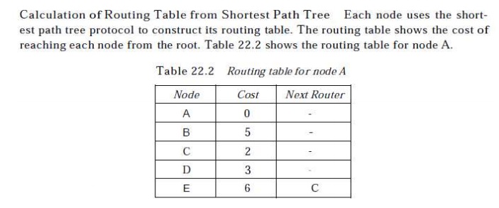
OSPF

The Open Shortest Path First or OSPF protocol is an intra domain routing protocol based on link state routing. Its domain is also an autonomous system. Areas To handle routing efficiently and in a timely manner, OSPF divides an autonomous system into areas. An area is a collection of networks, hosts, and routers all contained within an autonomous system. An autonomous system can be divided into many different areas.

All networks inside an area must be connected. Routers inside an area flood the area with routing information. At the border of an area, special routers called area border routers summarize the information about the area and send it to other areas. Among the areas inside an autonomous system is a special area called the backbone; all the areas inside an autonomous system must be connected to the backbone. In other words, the backbone serves as a primary area and the other areas as secondary areas.

This does not mean that the routers within areas cannot be connected to each other, however. The routers inside the backbone are called the backbone routers. Note that a backbone router can also be an area border router. If, because of some problem, the connectivity between a backbone and an area is broken, a virtual link between routers must be created by an administrator to allow continuity of the functions of the backbone as the primary area.Each area has an area identification. The area identification of the backbone is zero. Below Figure shows an autonomous system and its areas.

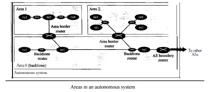
Areas in an autonomous system

Metric

The OSPF protocol allows the administrator to assign a cost, called the metric, to each route. The metric can be based on a type of service (minimum delay, maximum throughput, and so on). As a matter of fact, a router can have multiple routing tables, each based on a different type of service. Types of Links In OSPF terminology, a connection is called a link. Four types of links have been defined: point-to-point, transient, stub, and virtual.

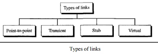
Types of links

A point-to-point link connects two routers without any other host or router in between. In other words, the purpose of the link (network) is just to connect the two routers. An example of this type of link is two routers connected by a telephone line or a T line. There is no need to assign a network address to this type of link. Graphically, the routers are represented by nodes, and the link is represented by a bidirectional edge connecting the nodes. The metrics, which are usually the same, are shown at the two ends, one for each direction.

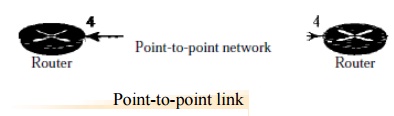
Point-to-point link

A transient link is a network with several routers attached to it. The data can enter through any of the routers and leave through any router. All LANs and some WANs with two or more routers are of this type. In this case, each router has many neighbors. For example, consider the Ethernet in Figure. Router A has routers B, C, D, and E as neighbors. Router B has routers A, C, D, and E as neighbors.

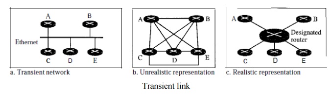
Transient link

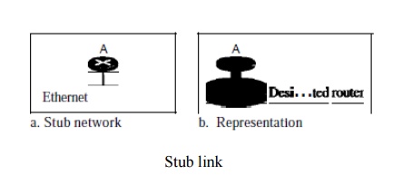
A stub link is a network that is connected to only one router. The data packets enter the network through this single router and leave the network through this same router. This is a special case of the transient network. We can show this situation using the router as a node and using the designated router for the network.

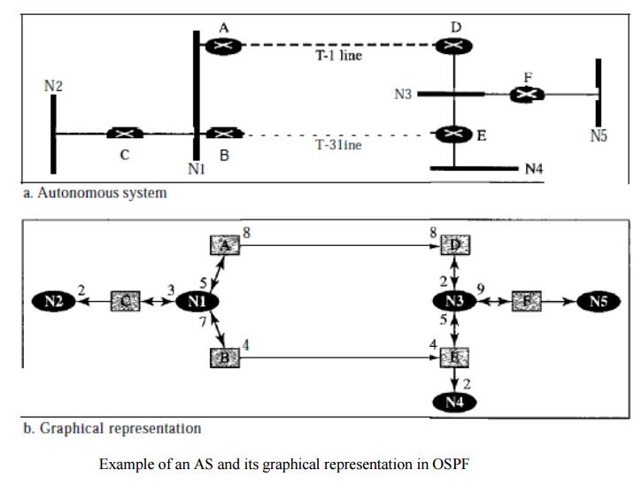
When the link between two routers is broken, the administration may create a virtual link between them, using a longer path that probably goes through several routers. Graphical Representation Let us now examine how an AS can be represented graphically. Figure shows a small AS with seven networks and six routers. Two of the networks are point-to-point networks. We use symbols such as Nl and N2 for transient and stub networks. There is no need to assign an identity to a point-to-point network. The figure also shows the graphical representation of the AS as seen by OSPF.

Distance Vector Routing Protocol

Routing Information Protocol (RIP) is an implementation of the distance vector protocol. Open Shortest Path First (OSPF) is an implementation of the link state protocol.

Border Gateway Protocol (BGP) is an implementation of the path vector protocol.

In distance vector routing, the least-cost route between any two nodes is the route with minimum distance. In this protocol, as the name implies, each node maintains a vector (table) of minimum distances to every node. The table at each node also guides the packets to the desired node by showing the next stop in the route (next-hop routing).

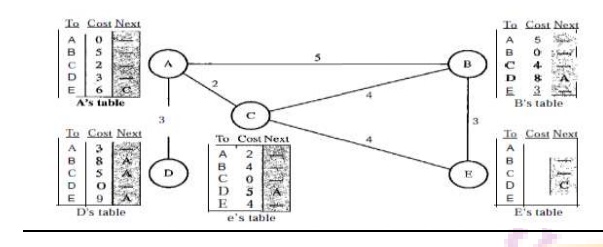
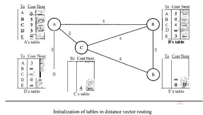
Distance vector routing tables

Initialization

The table for node A shows how we can reach any node from this node. For example, our least cost to reach node E is 6. The route passes through C. Each node knows how to reach any other node and the cost. Each node can know only the distance between itself and its immediate neighbors, those directly connected to it.

So for the moment, we assume that each node can send a message to the immediate neighbors and find the distance between itself and these neighbors.

Sharing - In distance vector routing, each node shares its routing table with its immediate neighbors periodically and when there is a change.

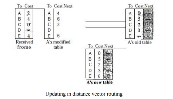
Updating - When a node receives a two-column table from a neighbor, it needs to update its routing table.

Updating takes three steps:

1. The receiving node needs to add the cost between itself and the sending node to each value in the second column. The logic is clear. If node C claims that its distance to a destination is x mi, and the distance between A and C is y mi, then the distance between A and that destination, via C, is x + y mi.

2.  The receiving node needs to add the name of the sending node to each row as the third column if the receiving node uses information from any row. The sending node is the next node in the route.

3. The receiving node needs to compare each row of its old table with the corresponding row of the modified version of the received table.

a. If the next-node entry is different, the receiving node chooses the row with the smaller cost. If there is a tie, the old one is kept.

b. If the next-node entry is the same, the receiving node chooses the new row. For example, suppose node C has previously advertised a route to node X with distance 3. Suppose that now there is no path between C and X; node C now advertises this route with a distance of infinity Node A must not ignore this value even though its old entry is smaller. The old route does not exist any more. The new route has a distance of infinity.

Each node can update its table by using the tables received from other nodes. When to Share:

Periodic Update A node sends its routing table, normally every 30 s, in a periodic update. The period depends on the protocol that is using distance vector routing.

Triggered Update A node sends its two-column routing table to its neighbors anytime there is a change in its routing table. This is called a triggered update.

The change can result from the following.

1. A node receives a table from a neighbor, resulting in changes in its own table after updating.

2.  A node detects some failure in the neighboring links which results in a distance change to infinity.

RIP

The Routing Information Protocol (RIP) is an intra-domain routing protocol used inside an autonomous system. It is a very simple protocol based on distance vector routing. RIP implements distance vector routing directly with some considerations:

1. In an autonomous system, we are dealing with routers and networks (links). The routers have routing tables; networks do not.

2.  The destination in a routing table is a network, which means the first column defines a network address.

3.  The metric used by RIP is very simple; the distance is defined as the number of links (networks) to reach the destination. For this reason, the metric in RIP is called a hop count.

4.  Infinity is defined as 16, which means that any route in an autonomous system using RIP cannot have more than 15 hops.

5. The next-node column defines the address of the router to which the packet is to be sent to reach its destination.