Constrained Problems: Equality Constraints

CONSTRAINED PROBLEMS

This section deals with the optimization of constrained continuous functions. Section 18.2.1 introduces the case of equality constraints and Section 18.2.2 deals with inequality constraints. The presentation in Section 18.2.1 is covered for the most part in Beightler and Associates (1979, pp. 45-55).

Equality Constraints

This section presents two methods: the Jacobian and the Lagcangean. The Lagrangean method can be developed logically from the Jacobian. This relationship provides an in-teresting economic interpretation of the Lagrangean method.

Constrained Derivatives (Jacobian) Method.   Consider the problem

The functions f(X) and g(X), i = 1,2, ... , m, are twice continuously differentiable. The idea of using constrained derivatives is to develop a closed-form expression for the first partial derivatives of f(X) at all points that satisfy the constraints g(X) = 0. TIle corresponding stationary points are identified as the points at which these partial derivatives vanish. The sufficiency conditions introduced in Section 18.1 can then be used to check the identity of stationary points.

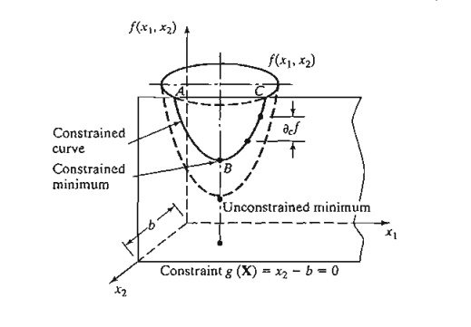
To clarify the proposed concept, consider f(x1, x2) illustrated in Figure 18.4. This function is to be minimized subject to the constraint

where b is a constant. From Figure 18.4, the curve designated by the three points A, B, and C represents the values of f(x1, x2) for which the given constraint is always satisfied. The constrained derivatives method defines the gradient of f(xl, x2) at any point on the curve ABC. Point B at which the constrained derivative vanishes is a stationary point for the constrained problem.

The method is now developed mathematically. By Taylor's theorem, for X + ΔX in the feasible neighborhood of X, we have

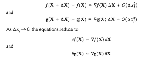
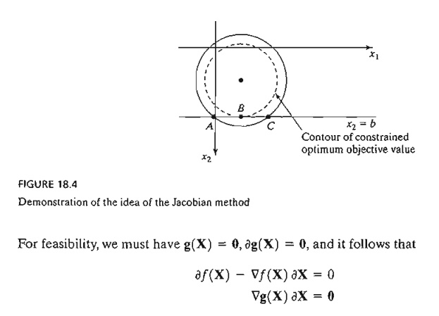
This gives (m + 1) equations in (n + 1) unknowns, ¶f(X) and ¶X. Note that ¶f(X) is a dependent variable, and hence is determined as soon as ¶X is known. This means that, in effect, we have m. equations in n unknowns.

If m > n, at least (m - n) equations are redundant. Eliminating redundancy, the system reduces to m ≤ n. If  m = n, the solution is ¶X = 0, and X has no feasible neighborhood, which means that the solution space consists of one point only. The remaining  case, where m < n, requires further elaboration.

Define

The vectors Y and Z are called the dependent and independent variables, respectively. Rewriting the gradient vectors of f and g in terms of Y and Z, we get

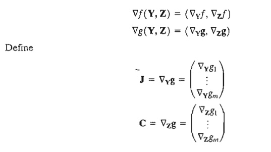
J mXm is called the Jacobian matrix and Cmxn-m the control matrix. The Jacobian J is assumed nonsingular. This is always possible because the given m equations are independent by definition. The components of the vector V must thus be selected from among those of X such that J is nonsingular.

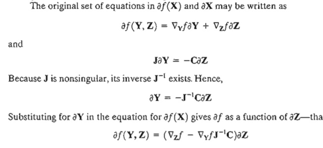
From this equation, the constrained derivative with respect to the independent vector Z is given by

where Ñcf is the constrained gradient vector of f with respect to Z. Thus, Ñcf (Y, Z) must be null at the stationary points.

The sufficiency conditions are similar to those developed in Section 18.1. The Hessian matrix will correspond to the independent vector Z, and the elements of the Hessian matrix must be the constrained second derivatives. To show how this is obtained, let

It thus follows that the ith row of the (constrained) Hessian matrix is a

 Notice that W is a function of Y and Y is a function of Z. Thus, the partial derivative of Ñcf with respect to zi is based on the following chain rule:

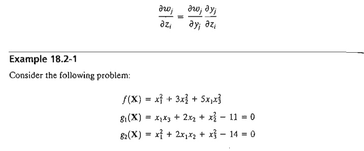
Given the feasible point XO = (1,2, 3), we wish to study the variation in f( = ¶cf) In the feasible neighborhood of X0.

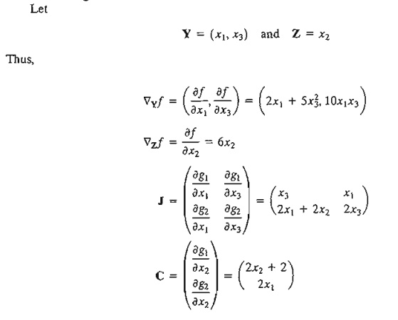
Suppose that we need to estimate ¶cf  in the feasible neighborhood of the feasible point Xo = (1,2,3) given a small change ¶x2 = .01 in the independent variable x2. We have

Hence, the incremental value of constrained f is given as

By specifying the value of ¶x2 for the independent variable x2, feasible values of ¶x1 and ¶x2 are determined for the dependent variables x1 and x3 using the formula

We now compare the value of ¶cf as computed above with the difference f(X o + ¶X) - f(X o), given ¶x2 = .01.

The amount -.477 compares favorably with ¶cf = -46.01¶x2 = - .4601. The difference between the two values is the result of the linear approximation in computing ¶cf at X0..

PROBLEM SET 18.2A

1. Consider Example 18.2-1.

a. Compute ¶cf by the two methods presented in the example, using ¶x2 = .001 instead of ¶x2 = .01. Does the effect of linear approximation become more negligible with the decrease in the value of ¶x2?

*(b) Specify a relationship among the elements of ¶x = (¶x1. ¶x2, ¶x3) at the feasible point X o = (1,2,3,) that will keep the point X o + ¶X feasible.

c. lf Y = (x2, x3) and Z = x1, what is the value of ¶x1 that will produce the same value of ¶cf given in the example?

Example 18.2-2

This example illustrates the use of constrained derivatives. Consider the problem

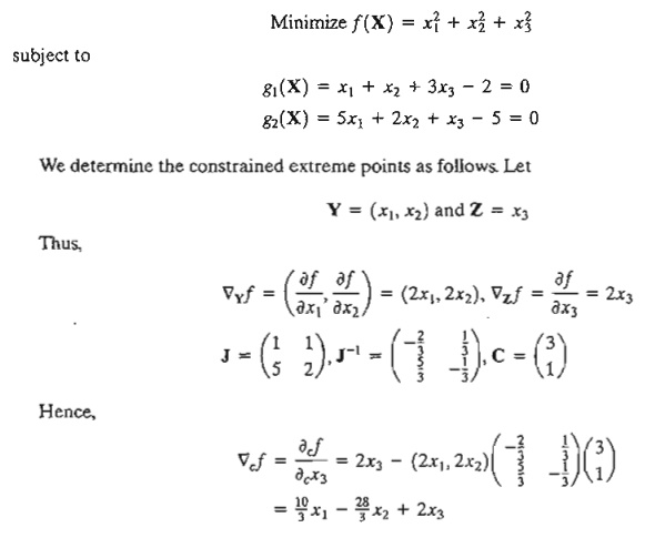
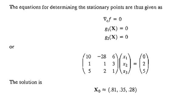
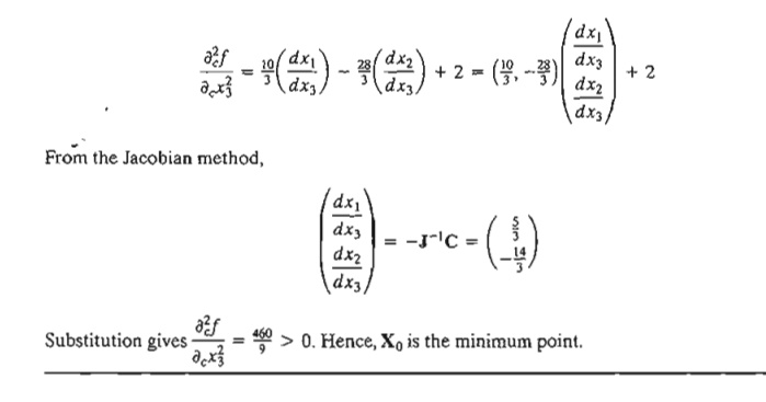
The identity of this stationary point is checked using the sufficiency condition. Given that x3 is the independent variable, it follows from Ñcf that

Sensitivity Analysis in the Jacobian Method. The Jacobian method can be used to study the effect of small changes in the right-hand side of the constraints on the optimal value of f Specifically, what is the effect of changing gi(X) = 0 to gi(X) = ¶gi on the optimal value of f? This type of investigation is called sensitivity analysis and is similar to that carried out in linear programming (see Chapters 3 and 4). However, sensitivity analysis in nonlinear programming is valid only in the small neighborhood of the extreme point. The development will be helpful in studying the Lagrangean method.

We have shown previously that

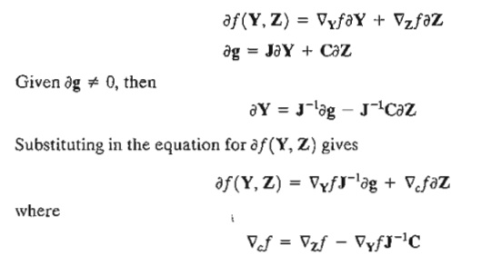
as defined previously. The expression for ¶ f(Y, Z) can be used to study variation in f in the feasible neighborhood of a feasible point X o resulting from small changes ¶g and ¶z.

At the extreme (indeed, any stationary) point Xo = (Yo, Zo) the constrained gradient Ñcf must vanish. Thus

The effect of the small change ¶g on the optimum value of f can be studied by evaluating the rate of change of f with respect to g. These rates are usually referred to as sensitivity coefficients.

Example 18.2-3

Consider the same problem of  Example 18.2-2.  The•  optimum point    is       given by Xo = (x01 x02, x03) = (.81, .35, .28). Given Yo =  (x01, x02), then

This means that for ¶gj = 1, f will increase approximately by .0867. Similarly, for ¶g2 = 1, f will increase approximately by .3067.

Application of the Jacobian Method to an LP Problem.      Consider the linear program

To account for the nonnegativity constraints xj ≥ 0, substitute xj = w2j. With this substitution, the nonnegativity conditions become implicit and the original problem becomes

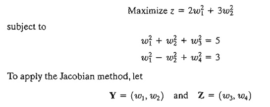
(In the terminology of linear programming, Y and Z correspond to the basic and non-basic variables, respectively.) Thus

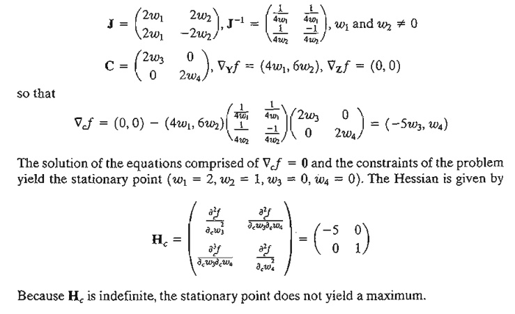
The reason the solution above does not yield the optimum solution is that the specific choices of Y and Z are not optimum. In fact, to find the optimum, we need to keep on altering our choices of Y and Z until the sufficiency condition is satisfied. This will be equivalent to locating the optimum extreme point of the linear programming solution space. For example, consider Y = (w2, w4) and Z = (w1, w3). The corresponding constrained gradient vector becomes

is negative-definite, the solution is a maximum point.

The result is verified graphically in Figure 18.5. The first solution (x1 = 4, x2 = 1) is not optimal, and the second (xl = 0, x2 = 5) is. You can verify that the remaining two (feasible) extreme points of the solution space are not optimal. In fact, the extreme point (x1 = 0, x2 = 0) can be shown by the sufficiency condition to yield a minimum point.

The sensitivity coefficients ÑY0fJ-1 when applied to linear programming yield the dual values. To illustrate this point for the given numerical example, let u1 and u2 be the corresponding dual variables. At the optimum point (w1 = 0, w2 = Rt(5), w3 = 0, w4 = Rt(8)), these dual variables are given by

The corresponding dual objective value is 5u1 + 3u2 = 15, which equals the optimal primal objective value. The given solution also satisfies the dual constraints and hence is optimal and feasible. This shows that the sensitivity coefficients are the same as the dual variables. In fact, both have the same interpretation.

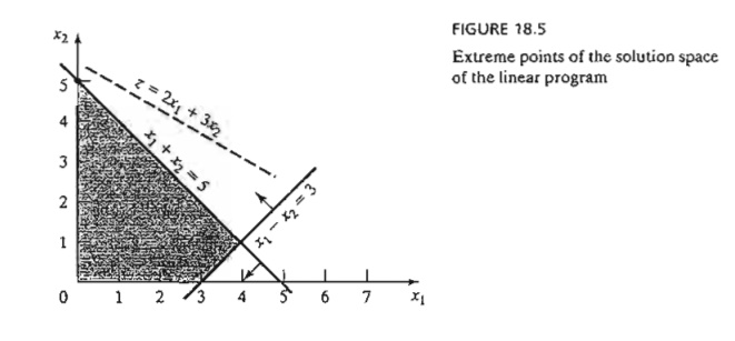
We can draw some general conclusions from the application of the Jacobian method to the linear programming problem. From the numerical example, the necessary conditions require the independent variables to equal zero. Also, the sufficiency conditions indicate that the Hessian is a diagonal matrix. Thus, all its diagonal elements must be positive for a minimum and negative for a maximum. The observations demonstrate that the necessary condition is equivalent to specifying that only basic (feasible) solutions are needed to locate the optimum solution. In this case the independent variables are equivalent to the nonbasic variables in the linear programming problem. Also, the sufficiency condition demonstrates the strong relationship between the diagonal elements of the Hessian matrix and the optimality indicator zj - cj (see Section 7.2) in the simplex method:

PROBLEM SET 18.2B

1. Suppose that Example 18.2-2 is solved in the following manner. First, use the constraints to express x1 and x2 in terms of x3. then use the resulting equations to express the objective function in terms of x3 only. By taking the derivative of the new objective function with respect to x3, we can determine the points of maxima and minima.

a.     Would the derivative of the new objective function (expressed in terms of x3) be different from that obtained by the Jacobian method?

b.     How does the suggested procedure differ from the Jacobian method?

2. Apply the Jacobian method to Example 18.2-1 by selecting Y = (x2,  x3)  and Z = (x1).

*3. Solve by the Jacobian method:

where C is a positive constant. Suppose that the right-hand side of the constraint is changed to C + δ, where δ is a small positive quantity. Find the corresponding change in the optimal value of f.

4. Solve by the Jacobian method:

(a) Find the change in the optimal value of f(X) if the constraint is replaced by x1x2 – 9.99 =0.

(b) Find the change in value of f (X) if the neighborhood of the feasible point (2,5) given that xIx2 = 9.99 and δ xl == .01.

 5. Consider the problem:

Apply the Jacobian method to find ¶f(X) in the neighborhood of the feasible point (1, 1; 1). Assume that this neighborhood is specified by ¶g1 = -.01, ¶g2 = .02, and ¶x1 = .01

6.    Consider the problem

(a) Show that by selecting x3 and x4 as independent variables, the Jacobian method fails to provide a solution and state the reason.

*(b) Solve the problem using x1 and x3 as independent variables and apply the sufficiency condition to determine the type of the resulting stationary point.

(c) Determine the sensitivity coefficients given the solution in (b).

7. Consider the linear programming problem.

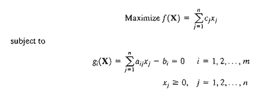
Neglecting the nonnegativity constraint, show that the constrained derivatives Ñcf(X) for this problem yield the same expression for {zj - cj} defined by the optimality condition of the linear programming problem (Section 7.2)-that is,

Can the constrained-derivative method be applied directly to the linear programming problem? Why or why not?

Lagrangean Method. In the Jacobian method, let the vector A represent the sensitivity coefficients-that is

This equation satisfies the necessary conditions for stationary points because ¶f/¶g is computed such that Ñcf = 0. A more convenient form for presenting these equations is to take their partial derivatives with respect to all xj. This yields

The resulting equations together with the constraint equations g(X) = 0 yield the feasible values of X and A that satisfy the necessary conditions for stationary points.

The given procedure defines the Lagrangean method for identifying the stationary points of optimization problems with equality constraints. Let

The function L is called the Lagrangean function and the parameters l the Lagrange multipliers. By definition, these multipliers have the same interpretation as the sensitivity coefficients of the Jacobian method.

The equations

give the necessary conditions for determining stationary points of f(X) subject to g(X) = 0. Sufficiency conditions for the Lagrangean method exist but they are generally computationally intractable.

Example 18.2-4

Consider the problem of Example 18.2-2. The Lagrangean function is

This yields the following necessary conditions:

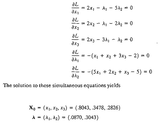
This solution combines the results of Examples 18.2-2 and 18.2-3. The values of the Lagrange multipliers l equal the sensitivity coefficients obtained in Example 18.2-3. The result shows that these coefficients are independent of the specific choice of the dependent vector Y in the Jacobian method.

PROBLEM SET 18.2C

1. Solve the following linear programming problem by both the Jacobian and the Lagrangean methods:

*2.     Find the optimal solution to the problem

Suppose that g1 (X) = .01 and g2(X) = .02. Find the corresponding change in the optimal value of f(X).

3. Solve Problem 6, Set 18.2b, by the Lagrangean method and verify that the values of the Lagrange multipliers are the same as the sensitivity coefficients obtained in Problem 6, Set 18.2b.