Properties, Procedure Steps, Example Solved Problems | Statistics - Chi-Square Distribution and Its Applications | 12th Statistics : Chapter 2 : Tests Based on Sampling Distributions I
Chapter: 12th Statistics : Chapter 2 : Tests Based on Sampling Distributions I
Chi-Square Distribution and Its Applications
CHI-SQUARE DISTRIBUTION AND ITS APPLICATIONS
Karl Pearson (1857-1936) was a English Mathematician and
Biostatistician. He founded the worldŌĆÖs first university statistics department
at University College, London in 1911. He was the first to examine whether the
observed data support a given specification, in a paper published in 1900. He
called it ŌĆśChi-square goodness of fitŌĆÖ test which motivated research in
statistical inference and led to the development of statistics as separate
discipline.
1. Chi-Square distribution
The square of standard normal variable is known as a chi-square
variable with 1 degree of freedom (d.f.). Thus
If X ~ N (┬Ą, Žā2), then it is known
that  ~ N 0,1 . Further Z2
is said to follow Žć2 ŌĆō distribution with 1 degree of freedom (Žć2
ŌĆō pronounced as chi-square)
~ N 0,1 . Further Z2
is said to follow Žć2 ŌĆō distribution with 1 degree of freedom (Žć2
ŌĆō pronounced as chi-square)
Note: i) If Xi ~ N (┬Ą, Žā2) , i = 1, 2, ŌĆ”, n are n iid random variables, then
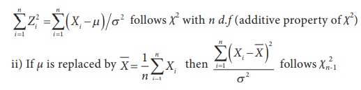
2. Properties of c2 distribution
It is a continuous distribution.
┬Ę
The distribution has only one parameter i.e. n d.f.
┬Ę
The shape of the distribution depends upon the d.f, n.
┬Ę
The mean of the chi-square distribution is n and variance 2n
┬Ę
If U and V are independent random variables having Žć2
distributions with degree of freedom n1 and n2
respectively, then their sum U + V has the same Žć2
distribution with d.f n1 + n2.
3. Applications of chi-square distribution
To test the variance of the normal population,
using the statistic in note (ii)
┬Ę
To test the independence of attributes.
┬Ę
To test the goodness of fit of a distribution.
┬Ę
The sampling distributions of the test statistics used in the last
two applications are approximately chi-square distributions.
4. Test of Hypotheses for population variance of the normal population (Population mean is assumed to be unknown)
Procedure
Step 1 : Let ┬Ą and Žā2 be
respectively the mean and the variance of the normal population under study,
where Žā2 is known and ┬Ą unknown. If Žā02
is an admissible value of Žā2, then frame the
Null hypothesis as H0: Žā
2 = Žā 02 and
choose the suitable alternative hypothesis from
(i) H1 : Žā2
ŌēĀ Žā02 (ii) H1
: Žā2 > Žā02 (iii) H1 : Žā2 < Žā02
Step 2 : Describe the sample/data and its descriptive measures. Let (X1,
X2, ŌĆ”, Xn) be a random sample
of n observations drawn from the population, where n is small (n
< 30).
Step 3 : Fix the desired level of significance ╬▒.
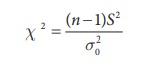
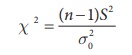
Step 4 : Consider
the test statistic 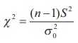 under H0. The approximate sampling
distribution of the test statistic under
H0 is the chi-square distribution with (nŌĆō1) degrees of freedom.
under H0. The approximate sampling
distribution of the test statistic under
H0 is the chi-square distribution with (nŌĆō1) degrees of freedom.
Step 5 : Calculate the value of the of Žć2 for the given
sample as 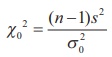
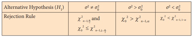
Step 6 : Choose the critical value of Žće2
corresponding to ╬▒ and H1 from
the following table.
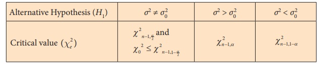
Step 7 : Decide on H0 choosing the suitable
rejection rule from the following table corresponding to H1.
Example 2.6
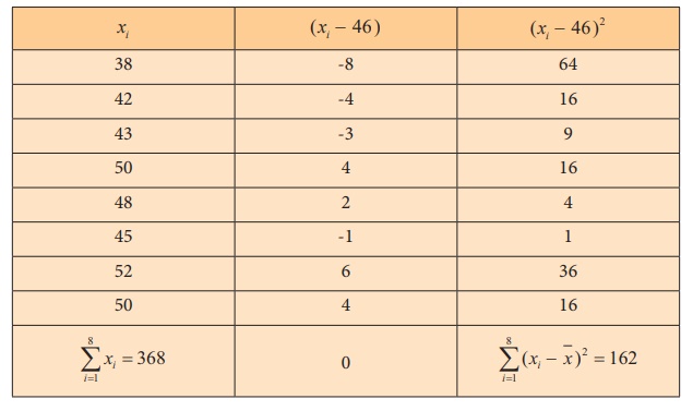
The weights (in kg.) of 8 students of class VII are 38, 42, 43,
50, 48, 45, 52 and 50. Test the hypothesis that the variance of the population
is 48 kg, assuming the population is normal and ┬Ą is unknown.
Solution:
Step 1 : Null Hypothesis H0: Žā2 = 48 kg.
i.e. Population variance can be regarded as 48 kg.
Alternative hypothesis H1: Žā2 ŌēĀ 48 kg.
i.e. Population variance cannot be regarded as 48 kg.
Step 2 : The given sample information is
Sample size (n)= 8
Step 3 : Level of significance
╬▒= 5%
Step 4 : Test statistic
Under null hypothesis H0
follows chi-square distribution with (nŌĆō1) d.f.
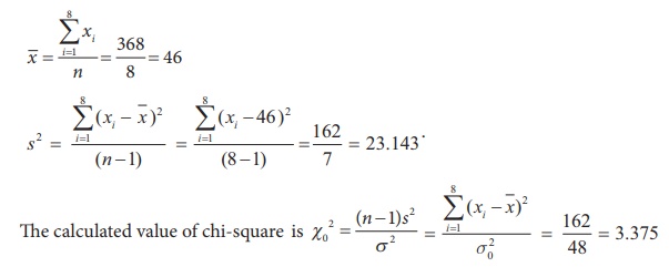
Step 5 : Calculation of test statistic
The value of chi-square under H0 is calculated
as under:
To find ![]() and sample variance s2,
we form the following table.
and sample variance s2,
we form the following table.
Step 6 : Critical values
Since H1 is a two sided alternative, the
critical values at ╬▒ =0.05 are Žć27, 0.025
= 16.01 and Žć27,0.975 = 1.69.
Step 7 : Decision
Since it is a two-tailed test, the elements of the
critical region are determined by the
rejection rule 1.69 = Žć27, 0.975 < Žć02 (=3.375) < Žć27,0.025 = 16.01.
For the given sample information, the rejection
rule does not hold, since
1.69 = Žć27,
0.975 < Žć02
(=3.375) < Žć27,0.025
= 16.01.
Hence, H0
is not rejected in favour of H1.
Thus, Population variance can be regarded as 48 kg.
Example 2.7
A normal population has mean ┬Ą (unknown) and variance 9. A
sample of size 9 observations has been taken and its variance is found to be
5.4. Test the null hypothesis H0: Žā2 = 9
against H1: Žā2 > 9 at 5% level of
significance.
Solution:
Step 1 : Null Hypothesis H0: Žā2 = 9.
i.e., Population variance regarded as 9.
Alternative hypothesis H1: Žā2 > 9.
i.e. Population variance is regarded as greater than 9.
Step 2 : Data
Sample size (n) = 9
Sample variance (s2) = 5.4
Step 3 : Level of significance
╬▒ = 5%
Step 4 : Test statistic
Under null hypothesis H0
follows
chi-square distribution with (n-1)
degrees of freedom.
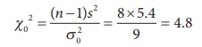
Step 5 : Calculation of test statistic
The value of chi-square under H0 is calculated
as
Step 6 : Critical value
Since H1 is a one-sided alternative, the
critical values at ╬▒ =0.05 is Žće2 = Žć28,
0.05 = 15.507.
Step 7 : Decision
Since it is a one-tailed test, the elements of the critical region
are determined by the rejection rule Žć02 > Žće2.
For the given sample information, the rejection rule does not hold , since Žć02 = 4.8 < Žć28, 0.05 = 15.507. Hence, H0 is not rejected in favour of H1. Thus, the population variance can be regarded as 9.
Example 2.8
A normal population has mean ┬Ą (unknown) and variance
0.018. A random sample of size 20 observations has been taken and its variance
is found to be 0.024. Test the null hypothesis H0: Žā2
= 0.018 against H1: Žā2 <
0.018 at 5% level of significance.
Solution:
Step 1 : Null Hypothesis H0: Žā2 = 0.018.
i.e. Population variance regarded as 0.018.
Alternative hypothesis H1: Žā2 < 0.018.
i.e. Population variance is regarded as lessthan 0.018.
Step 2 : Data
Sample size (n) = 20
Sample variance (s2) = 0.024
Step 3 : Level of significance
╬▒= 5%
Step 4 : Test statistic
Under null hypothesis H0
follows
chi-square distribution with (nŌĆō1)
degrees of freedom.
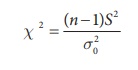
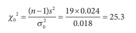
Step 5 : Calculation of test statistic
The value of chi-square under H0 is calculated
as
Step 6 : Critical value
Since H1 is a one-sided alternative, the
critical values at ╬▒ =0.05 is Žće2 = Žć219,
0.95 = 10.117.
Step 7 : Decision
Since it is a one-tailed test, the elements of the critical region
are determined by the rejection rule Žć02 < Žće2
For the given sample information, the rejection rule does not
hold, since Žć02 = 25.3 > Žće2
= Žć219, 0.95 = 10.117.
Hence, H0 is not rejected in favour of H1
. Thus, the population variance can be regarded as 0.018.
5. Test of Hypotheses for independence of Attributes
Another important application of Žć2 test is the
testing of independence of attributes.
Attributes: Attributes are qualitative characteristic such as levels of
literacy, employment status, etc., which are quantified in terms
of levels/scores.
Contigency table: Independence of two attributes is an important
statistical application in which the data pertaining to the attributes
are cross classified in the form of a two ŌĆō dimensional table. The levels of
one attribute are arranged in rows and of the other in columns. Such an
arrangement in the form of a table is called as a contingency table.
Computational steps for testing the independence of attributes:
Step 1 : Framing the hypotheses
Null hypothesis H0: The two attributes are independent
Alternative hypothesis H1: The two attributes are not independent.
Step 2 : Data
The data set is given in the form of a contigency as under.
Compute expected frequencies Eij corresponding to each cell
of the contingency table, using the formula
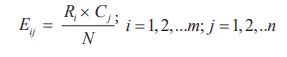
where,
N = Total sample size
Ri = Row sum corresponding to ith row
C j
= Column
sum corresponding to jth column
Step
3 :
Level of significance
Fix the desired level of significance ╬▒
Step
4 :
Calculation
Calculate the value of the test statistic as
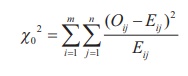
Step
5 :
Critical value
The critical value is obtained from the table of Žć2 with (mŌĆō1)(nŌĆō1) degrees of freedom
at given level of significance, ╬▒ as Žć2(mŌĆō1)(nŌĆō1), ╬▒.
Step
6 :
Decision
Decide on rejecting or not rejecting the null
hypothesis by comparing the calculated value of the test statistic with the
table value. If Žć02
Ōēź Žć2(mŌĆō1)(nŌĆō1),
╬▒ reject H0.
Note:
┬Ę
N, the total frequency should be
reasonably large, say greater than 50.
┬Ę
No theoretical cell-frequency should
be less than 5. If cell frequencies are less than 5, then it should be grouped
such that the total frequency is made greater than 5 with the preceding or
succeeding cell.
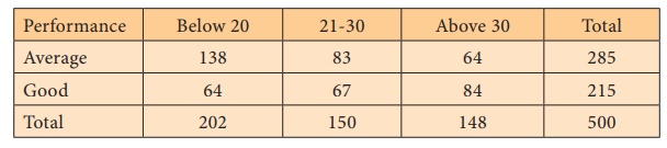
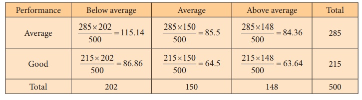
Example 2.9
The following table gives the performance of 500 students
classified according to age in a computer test. Test whether the attributes age
and performance are independent at 5% of significance.
Solution:
Step 1 : Null hypothesis H0: The attributes age and performance are
independent.
Alternative hypothesis H1: The attributes age and performance are not
independent.
Step 2 : Data
Compute expected frequencies Eij corresponding
to each cell of the contingency table, using the formula
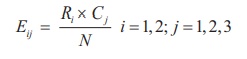
where,
N = Total sample size
Ri = Row sum corresponding to ith row
Cj = Column sum corresponding to jth column
Step 3 : Level of significance
╬▒ = 5%
Step 4 : Calculation
Calculate the value of the test statistic as
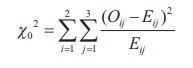
This chi-square test statistic is calculated as
follows:
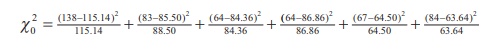
= 22.152 with degrees of freedom (3ŌĆō1)(2ŌĆō1) = 2
Step 5 : Critical value
From the chi-square table
the critical value
at 5% level
of significance is Žć2 (2-1)(3-1), 0.05
= Žć 22 ,
0.05 = 5.991.
Step 6 : Decision
As the calculated value Žć02 = 22.152 is greater
than the critical value Žć2 2005 = 5.991
the null hypothesis H0 is
rejected. Hence, the performance and age of students are not independent.
The following example will illustrate the procedure
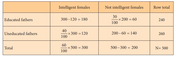
Example 2.10
A survey was conducted with 500 female students of which 60% were
intelligent, 40% had uneducated fathers, while 30 % of the not intelligent
female students had educated fathers. Test the hypothesis that the education of
fathers and intelligence of female students are independent.
Solution:
Step 1 : Null hypothesis H0: The attributes are independent i.e.
No association between education fathers and intelligence of female
students
Alternative hypothesis H1: The attributes are not independent i.e there is association between education of
fathers and intelligence of female students
Step 2 : Data
The observed frequencies (O) has been computed from the
given information as under.
Step 3 : Level of significance
╬▒ = 5%
Step 4 : Calculation
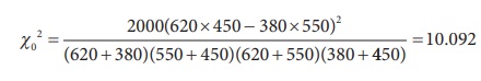
Calculate the value of the test statistic as
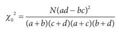
where,
a= 620, b = 380, c = 550, d = 450 and N = 2000
Step 5 : Critical value
From chi-square table the critical value at 5%
level of significance is Žć 21,
0.05 = 3.841
Step 6 : Decision
The calculated value Žć 20 = 10.092 is greater than the critical value Žć 21, 0.05 = 3.841, the null hypothesis H0 is rejected. Hence, education of fathers and intelligence of female students are not independent.
6. Tests for Goodness of Fit
Another important application of chi-square distribution is
testing goodness of a pattern or distribution fitted to given data. This
application was regarded as one of the most important inventions in mathematical
sciences during 20th century. Goodness of fit indicates the closeness of
observed frequency with that of the expected frequency. If the curves of these
two distributions do not coincide or appear to diverge much, it is noted that
the fit is poor. If two curves do not diverge much, the fit is fair.
Computational steps for testing the significance of goodness of fit:
Step 1 : Framing of hypothesis
Null hypothesis H0 : The goodness of fit is appropriate for the
given data set
Alternative hypothesis H1 : The goodness of fit is not appropriate for the
given data set
Step 2 : Data
Calculate the expected frequencies (Ei) using
appropriate theoretical distribution such as Binomial or Poisson.
Step 3 : Select the desired level of significance ╬▒
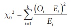
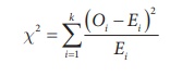
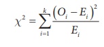
Step 4 : Test statistic
The test statistic is
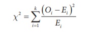
where
k = number of classes
Oi
and Ei are respectively the observed and expected frequency of
ith class such that
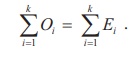
If any of Ei is found less than 5, the
corresponding class frequency may be pooled with preceding or succeeding
classes such that Ei's of all classes are greater than or
equal to 5. It may be noted that the value of k may be determined after
pooling the classes.
The approximate sampling distribution of the test statistic under H0
is the chi-square distribution with k-1-s d.f , s being the
number of parametres to be estimated.
Step 5 : Calculation
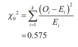
Calculate the value of chi-square as
The above steps in calculating the chi-square can be summarized in
the form of the table as follows:
Step 6 : Critical value
The critical value is obtained from the table of Žć2
for a given level of significance ╬▒.
Step 7 : Decision
Decide on rejecting or not rejecting the null hypothesis by
comparing the calculated value of the test statistic with the table value, at
the desired level of significance.
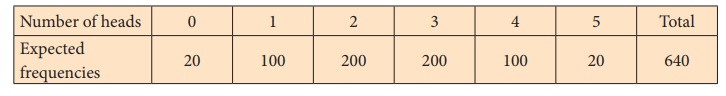
Example 2.11
Five coins are tossed 640 times and the following results were
obtained.
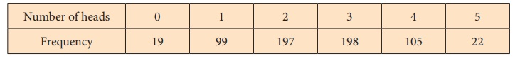
Fit binomial distribution to the above data.
Solution:
Step 1 : Null hypothesis H0: Fitting of binomial distribution is
appropriate for the given data.
Alternative hypothesis H1: Fitting of binomial distribution is not
appropriate to the given data.
Step 2 : Data
Compute the expected frequencies:
n = number of coins tossed at a time = 5
Let X denote the number of heads (success) in n
tosses
N = number of times experiment is repeated = 640
To find mean of the distribution
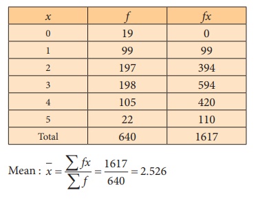
The probability mass function of binomial
distribution is :
p(x) = nCx
px qnŌĆōx, x = 0,1,...,
n (2.1)
Mean of the binomial distribution is ![]() = np.
= np.
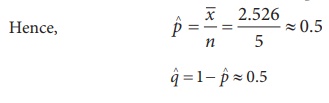
For x =
0, the equation (2.1) becomes
P(X = 0) = P(0) = 5c0 (0.5)5 = 0.03125
The expected frequency at x = N P(x)
The expected frequency at x =0 : N ├Ś P(0)
= 640 ├Ś 0.03125
= 20
We use recurrence formula to find the other
expected frequencies.
The expected frequency at x+1 is
 ├Ś
Expected frequency at x
├Ś
Expected frequency at x
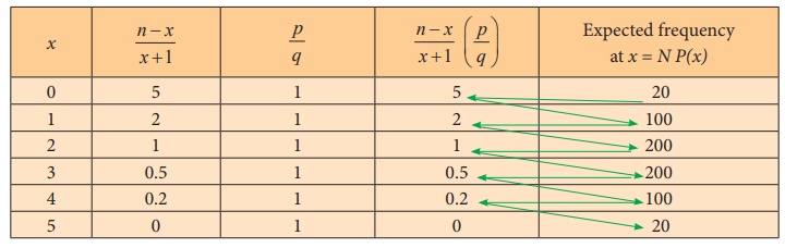
Table of expected frequencies:
Step 3 : Level of significance
╬▒= 5%
Step 4 : Test statistic
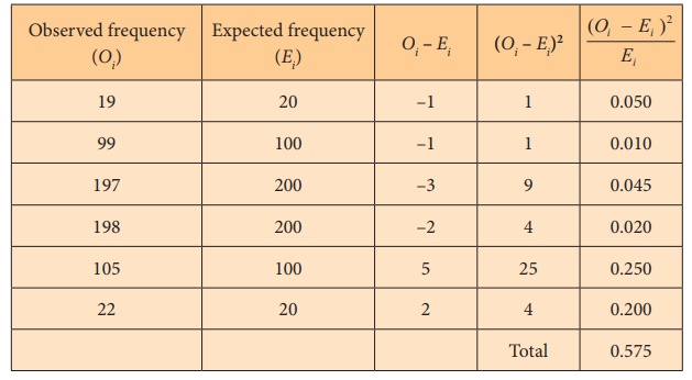
Step 5 : Calculation
The test statistic is computed as under:
Step 6 : Critical value
Degrees of freedom = k ŌĆō 1 ŌĆō s = 6 ŌĆō 1 ŌĆō 1 = 4
Critical value for d.f 4 at 5% level of significance is
9.488 i.e., c42, 0.05 = 9.488
Step 7 : Decision
As the calculated Žć 0 2 (=0.575) is less than the critical value Žć24, 0.05 = 9.488, we do not reject the null hypothesis. Hence, the fitting of binomial distribution is appropriate.
Example 2.12
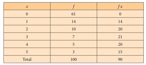
A packet consists of 100 ball pens. The distribution of the number
of defective ball pens in each packet is given below:

Examine whether Poisson distribution is appropriate for the above
data at 5% level of significance.
Solution:
Step 1 : Null hypothesis H0: Fitting of Poisson distribution is appropriate
for the given data.
Alternative hypothesis H1: Fitting of Poisson distribution is not
appropriate for the given data.
Step 2 : Data
The expected frequencies are computed as under:
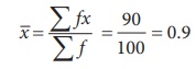
To find the mean of the distribution.
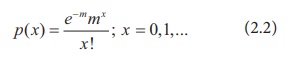
Probability
mass function of Poisson distribution is:
In
the case of Poisson distribution mean (m)
= ![]() = 0.9.
= 0.9.
At
x = 0, equation (2.2) becomes
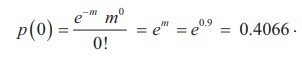
The
expected frequency at x is N P(x)
Therefore, The expected frequency at 0 is
N ├Ś P (0)
= 100 ├Ś 0.4066
= 40.66
We use recurrence formula to find the other
expected frequencies.
The expected frequency at x+1 is
[ m / x+1 ] ├Ś Expected frequency at x
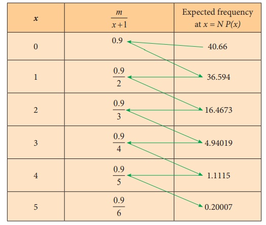
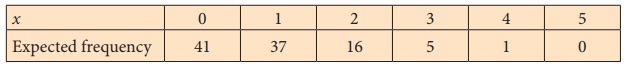
Table
of expected frequency distribution (on rounding to the nearest integer)
Step 3 : Level of significance
╬▒ = 5%
Step 4 : Test statistic
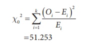
Step 5 : Calculation
The test statistic is computed as under:
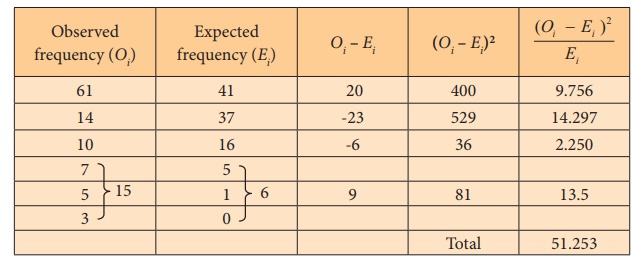
Note: In the above table, we find the cell
frequencies 0,1 in the expected frequency column (E) is less than 5, Hence, we combine (pool) with either succeeding
or preceding one such that the total is made greater than 5. Here we have
pooled with preceding frequency 5 such that the total frequency is made greater
than 5. Correspondingly, cell frequencies in observed frequencies are pooled.
Step 6 : Critical value
Degrees of freedom = (k ŌĆō 1 ŌĆō s) = 4 ŌĆō 1 ŌĆō 1 = 2
Critical value for 2 d.f at 5% level of significance is
5.991 i.e., Žć22, 0.05 = 5.991
Step 7 : Decision
The calculated Žć02 (=51.253) is greater than the critical value (5.991) at 5% level of significance. Hence, we reject H0. i.e., fitting of Poisson distribution is not appropriate for the given data.
Example 2.13
A sample 800 students appeared for a competitive examination. It
was found that 320 students have failed, 270 have secured a third grade, 190
have secured a second grade and the remaining students qualified in first
grade. The general opinion that the above grades are in the ratio 4:3:2:1
respectively. Test the hypothesis the general opinion about the grades is
appropriate at 5% level of significance.
Step 1 : Null hypothesis H0: The result in four grades follows the ratio
4:3:2:1
Alternative hypothesis H1: The result in four grades does not follows the
ratio 4:3:2:1
Step 2 : Data
Compute expected frequencies:
Under the assumption on H0, the expected frequencies of the four grades are:
4/10 ├Ś 800 = 320 ; 3/10 ├Ś 800 = 240; 2/10 ├Ś 800 =
160; 1/10 ├Ś 800 =80
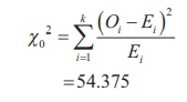
Step 3 : Test statistic
The test statistic is computed using the following table.
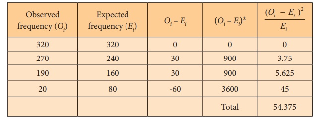
The test statistic is calculated as
Step 4 : Critical value
The critical value of Žć2 for 3 d.f. at 5% level
of significance is 7.81 i.e., Žć 23,
0.05 = 7.81
Step 5 : Decision
As the calculated value of Žć 02
(=54.375) is greater than the critical value Žć2 3, 0.05
= 7.81, reject H0.
Hence, the results of the four grades do not follow the ratio 4:3:2:1.
Example 2.14
The following table shows the distribution of digits in numbers
chosen at random from a telephone directory.

Test whether the occurence of the digits in the directory are
equal at 5% level of significance.
Step 1 : Null hypothesis H0: The occurrence of the digits are equal in the
directory.
Alternative hypothesis H1: The occurrence of the digits are not equal in
the directory.
Step 2 : Data
The expected frequency for each digit = 10000/10 = 1000
Step 3 : Level of significance
╬▒ = 5%
Step 4 : Test statistic
The test statistic is computed using the following table.
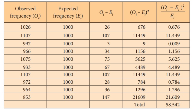
The test statistic is calculated as
Step
4 :
Critical value
Critical value for 9 df at 5% level of significance
is 16.919 i.e., Žć29, 0.05 = 16.919
Step
5 :
Decision
Since the calculated Žć02 (58.542) is greater than the critical
value Žć29, 0.05 = 16.919, reject H0. Hence, the digits are not uniformly distributed in
the directory.
Related Topics