Student’s t Distribution and Its Applications

STUDENT’S t DISTRIBUTION AND ITS APPLICATIONS

1. Student’s t-distribution

If X~N(0,1) and Y~χ_n² are independent random variables, then

is said to have t-distribution with n degrees of freedom. This can be denoted by t_n.

Note 1: The degrees of freedom of t is the same as the degrees of freedom of the corresponding chi-square random variable.

Note 2: The t-distribution is used as the sampling distribution(s) of the statistics(s) defined based on random sample(s) drawn from normal population(s).

(i) If X₁, X₂ , …, X_n is a random sample drawn from N (μ, σ²) population then

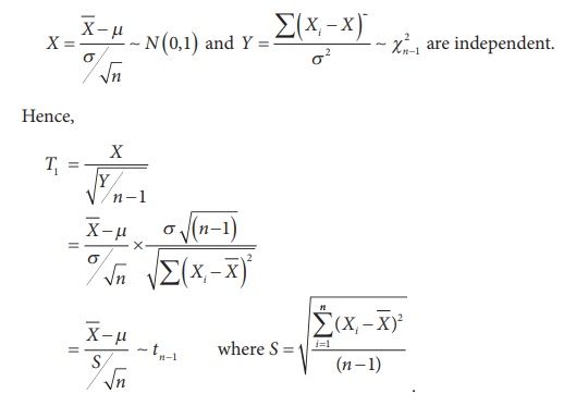
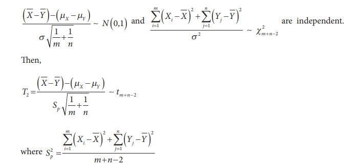
(ii) If (X₁ , X₂ , …, X_m) and (Y₁ , Y₂ , …, Y_n) are independent random samples drawn from N (μ_X , σ²) and N (μ_Y , σ²) populations respectively, then

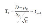
(iii) If (X₁ , Y₁), (X₂ , Y₂), …, (X_n , Y_n) is a random sample of n paired observations drawn from a bivariate normal population, then D_i = X_i – Y_i , i = 1, 2, …, n is a random sample drawn from N (μ_D , σ_D²). Here μ_D = μ_X – μ_Y.

Hence,

2. Properties of the Student’s t-distribution

1. t–distribution is symmetrical distribution with mean zero.

2. The graph of t-distribution is similar to normal distribution except for the following two reasons:

(i) The normal distribution curve is higher in the middle than t-distribution curve.

(ii) t–distribution has a greater spread sideways than the normal distribution curve. It means that there is more area in the tails of t-distribution.

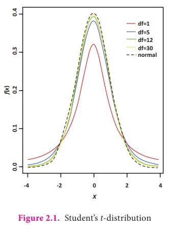
3. The t-distribution curve is asymptotic to X-axis, that is, it extends to infinity on either side.

4. The shape of t-distribution curve varies with the degrees of freedom. The larger is the number of degrees of freedom, closeness of its shape to standard normal distribution (fig. 2.1).

5. Sampling distribution of t does not depend on population parameter. It depends on degrees of freedom (n–1).

3. Applications of t-distribution

The t-distribution has the following important applications in testing the hypotheses for small samples.

1. To test significance of a single population mean, when population variance is unknown, using T₁.

2. To test the equality of two population means when population variances are equal and unknown, using T₂.

3. To test the equality of two means – paired t-test, based on dependent samples, T₃.

4. Test of Hypotheses for Normal Population Mean (Population Variance is Unknown)

Procedure:

Step 1 : Let µ and σ² be respectively the mean and variance of the population under study, where σ² is unknown. If µ₀ is an admissible value of µ, then frame the null hypothesis as

H₀: µ = µ₀ and choose the suitable alternative hypothesis from

(i) H₁: µ ≠ µ₀ (ii) H₁: µ > µ₀ (iii) H₁: µ < µ₀

Step 2 : Describe the sample/data and its descriptive measures. Let ( X₁, X₂, …, X_n) be a random sample of n observations drawn from the population, where n is small (n < 30).

Step 3 : Specify the level of significance, α.

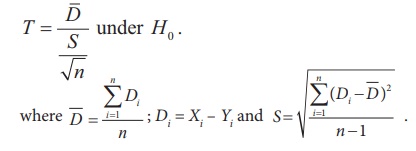
Step 4 : Consider the test statistic , under H₀, where  and S are the sample mean and sample standard deviation respectively. The approximate sampling distribution of the test statistic under H₀ is the t-distribution with (n–1) degrees of freedom.

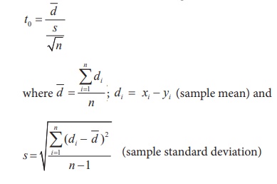
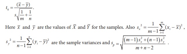
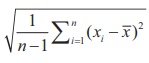Step 5 : Calculate the value of t for the given sample ( x₁ , x₂ ,... x_n ) as . here  is the sample mean and s =  is the sample standard deviation.

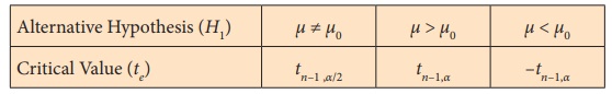
Step 6 : Choose the critical value, t_e, corresponding to α and H₁ from the following table

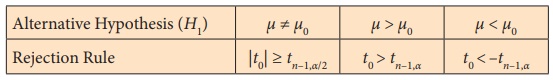
Step 7 : Decide on H₀ choosing the suitable rejection rule from the following table corresponding to H₁.

Example 2.1

The average monthly sales, based on past experience of a particular brand of tooth paste in departmental stores is ₹ 200. An advertisement campaign was made by the company and then a sample of 26 departmental stores was taken at random and found that the average sales of the particular brand of tooth paste is ₹ 216 with a standard deviation of ₹8. Does the campaign have helped in promoting the sales of a particular brand of tooth paste?

Solution:

Step 1 : Hypotheses

Null Hypothesis H₀: µ = 200

i.e., the average monthly sales of a particular brand of tooth paste is not significantly different from ₹ 200.

Alternative Hypothesis H₁: µ > 200

i.e., the average monthly sales of a particular brand of tooth paste are significantly different from ₹ 200. It is one-sided (right) alternative hypothesis.

Step 2 : Data

The given sample information are:

Size of the sample (n) = 26. Hence, it is a small sample.

Sample mean ( ) = 216, Standard deviation of the sample = 8.

Step 3 : Level of significance

α = 5%

Step 4 : Test statistic

The test statistic under H₀ is T = 

Since n is small, the sampling distribution of T is the t-distribution with (n–1) degrees of freedom.

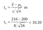
Step 5 : Calculation of test statistic

The value of T for the given sample information is calculated from

Step 6 : Critical value

Since H₁ is one-sided (right) alternative hypothesis, the critical value at α =0.05 is

t_e = t_{n-1, α} =t_25,0.05 = 1.708

Step 7 : Decision

Since it is right-tailed test, elements of critical region are defined by the rejection rule t₀ >t_e = t_{n-1, α} = t_25,0.05 = 1.708. For the given sample information t₀ = 10.20 > t_e =1.708. It indicates that given sample contains sufficient evidence to reject H₀. Hence, the campaign has helped in promoting the increase in sales of a particular brand of tooth paste.

Example 2.2

A sample of 10 students from a school was selected. Their scores in a particular subject are 72, 82, 96, 85, 84, 75, 76, 93, 94 and 93. Can we support the claim that the class average scores is 90?

Solution:

Step 1 : Hypotheses

Null Hypothesis H₀: µ = 90

i.e., the class average scores is not significantly different from 90.

Alternative Hypothesis H₁ : µ ≠ 90

i.e., the class means scores is significantly different from 90.

It is a two-sided alternative hypothesis.

Step 2 : Data

The given sample information are

Size of the sample (n) = 10. Hence, it is a small sample.

Step 3 : Level of significance

 α= 5%

Step 4 : Test statistic

The test statistic under H₀ is T =  

Since n is small, the sampling distribution of T is the t - distribution with (n–1) degrees of freedom.

Step 5 : Calculation of test statistic

The value of T for the given sample information is calculated from t₀ =  as under:

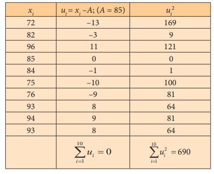
Sample mean

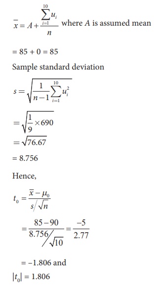
Step 6 : Critical value

Since H₁ is two-sided alternative hypothesis, the critical value at α  = 0.05 is t_e = t_{n-1, α/2} = t_9,0.025 = 2.262

Step 7 : Decision

Since it is two-tailed test, elements of critical region are defined by the rejection rule |t₀| > t_e = t _{n-1, α/2} = t =2.262. For the given sample information |t₀| = 1.806 < t_e = 2.262.

It indicates that given sample does not provide sufficient evidence to reject H₀. Hence, we conclude that the class average scores is 90.

5. Test of Hypotheses for Equality of Means of Two Normal Populations (Independent Random Samples)

Procedure:

Step 1 : Let μ_X and μ_Y be respectively the means of population-1 and population-2 under study. The variances of the population-1 and population-2 are assumed to be equal and unknown given by σ².

Frame the null hypothesis as H₀ : µ_X = µ_Y and choose the suitable alternative hypothesis from (i) H₁ : μ_X ≠ μ_Y (ii) H₁ : μ_X > μ_Y (iii) H₁ : μ_X < μ_Y

Step 2 : Describe the sample/data. Let (X₁, X₂ , …, X_m) be a random sample of m observations drawn from Population-1 and (Y₁, Y₂ , …, Y_n) be a random sample of n observations drawn from Population-2, where m and n are small (i.e., m < 30 and n < 30). Here, these two samples are assumed to be independent.

Step 3 : Set up level of significance (α)

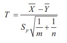
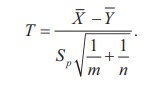
Step 4 : Consider the test statistic

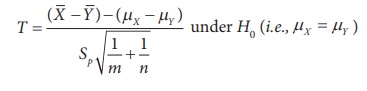
where S_p is the “pooled” standard deviation (combined standard deviation) given by

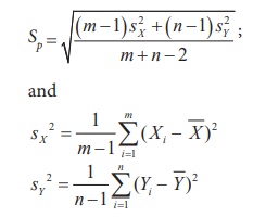
The approximate sampling distribution of the test statistic

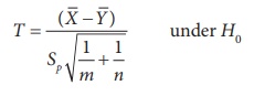
 is the t-distribution with m+n–2 degrees of freedom i.e., t ~ t_m+n–2.

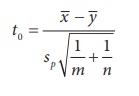
Step 5 : Calculate the value of T for the given sample ( x₁ , x₂ ,... x_m ) and ( y₁ , y ₂ ,... y_n ) as

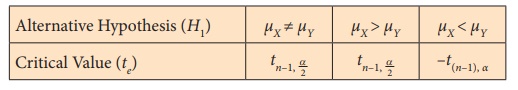
Step 6 : Choose the critical value, t_e, corresponding to α and H₁ from the following table

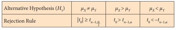
Step 7 : Decide on H₀ choosing the suitable rejection rule from the following table corresponding to H₁.

Example 2.3

The following table gives the scores (out of 15) of two batches of students in an examination.

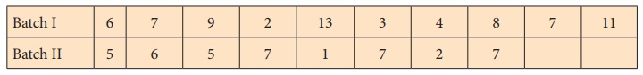
Test at 1% level of significance the average performance of the students in Batch I and Batch II are equal.

Solution:

Step 1 : Hypotheses: Let µ_X and µ_Y denote respectively the average performance of students in Batch I and Batch II. Then the null and alternative hypotheses are :

Null Hypothesis H₀ : µ _X = µ_Y

i.e., the average performance of the students in Batch I and Batch II are equal.

Alternative Hypothesis H₁ : µ _X ≠ µ_Y

i.e., the average performance of the students in Batch I and Batch II are not equal.

Step 2 : Data

The given sample information are:

Sample size for Batch I : m =10

Sample size for Batch II : n = 8

Step 3 : Level of significance

α= 1%

Step 4 : Test statistic

The test statistic under H₀ is

The sampling distribution of T under H₀ is the t-distribution with m+n–2 degrees of freedom i.e., t ~ t_m+n–2

Step 5 : Calculation of test statistic

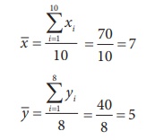
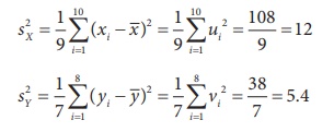
To find sample mean and sample standard deviation:

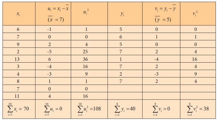
To find sample means:

Let (x₁ , x₂ ,..., x₁₀) and (y₁, y₂ ,..., y₈) denote the scores of students in Batch I and Batch II respectively.

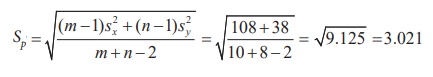
To find combined sample standard deviation:

Pooled standard deviation is:

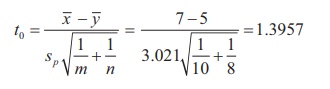
The value of T is calculated for the given information as

Step 6 : Critical value

Since H₁ is two-sided alternative hypothesis, the critical value at α = 0.01 is t_e = t_{m+n-2, α/2} = t_16,0.005 = 2.921

Step 7 : Decision

Since it is two-tailed test, elements of critical region are defined by the rejection rule |t₀| < t_e = t_m+n-2, α = t_16,0.005 = 2.921. For the given sample information |t₀| = 1.3957 < t_e = 2.921.

It indicates that² given sample contains insufficient evidence to reject H₀. Hence, the mean performance of the students in these batches are equal.

Example 2.4

Two types of batteries are tested for their length of life (in hours). The following data is the summary descriptive statistics.

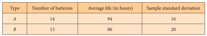
Is there any significant difference between the average life of the two batteries at 5% level of significance?

Solution:

Step 1 : Hypotheses

Null Hypothesis H₀ : μ_X = μ_Y

i.e., there is no significant difference in average life of two types of batteries A and B.

Alternative Hypothesis H₀ : μ_X ≠ μ_Y

i.e., there is significant difference in average life of two types of batteries A and B. It is a two-sided alternative hypothesis

Step 2 : Data

The given sample information are :

m = number of batteries under type A = 14

n = number of batteries under type B = 13

 = Average life (in hours) of type A battery = 94

 = Average life (in hours) of type B battery = 86

s_X = standard deviation of type A battery =16

s_Y = standard deviation of type B battery = 20

Step 3 : Level of significance

 α= 5%

Step 4 : Test statistic

The test statistic under H₀ is

The sampling distribution of T under H₀ is the t-distribution with m+n–2 degrees of freedom i.e., t ~ t_m+n–2

Step 5 : Calculation of test statistic

Under null hypotheses H₀:

where s is the pooled standard deviation given by,

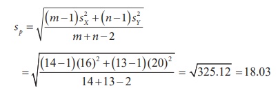
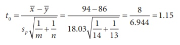
The value of T is calculated for the given information as

Step 6 : Critical value

Since H₁ is two-sided alternative hypothesis, the critical value at α = 0.05 is t_e = t_{m+n-2, α/2} = t_{25, 0.025} = 2.060.

Step 7 : Decision

Since it is a two-tailed test, elements of critical region are defined by the rejection rule |t₀| < t_e = t_m+n-2,α/2 = t_{25, 0.025} = 2.060. For the given sample information |t₀| = 1.15 < t_e = 2.060. It indicates that2 given sample contains insufficient evidence to reject H0. Hence, there is no significant difference between the average life of the two types of batteries.

6. To test the equality of two means – paired t-test

Procedure:

Step 1 : Let X and Y be two correlated random variables having the distributions respectively N(μ_X , σ_X²) (Population-1) and N(μ_Y , σ_Y²) (Population-2). Let D = X–Y, then it has normal distribution N(μ_D = μ_X – μ_Y, σ_D²).

Frame null hypothesis as

H₀ : μ_D= 0

And choose alternative hypothesis from

(i) H₁ : μ_D≠ 0 (ii) H₁ : μ_D> 0 (iii) H₁ : μ_D< 0

Step 2 : Describe the sample/data. Let (X₁, X₂, …, X_m) be a random sample of m observations drawn from Population-1 and (Y₁, Y₂, …, Y_n) be a random sample of n observations drawn from Population-2. Here, these two samples are correlated in pairs.

Step 3 : Set up level of significance (α)

Step 4 : Consider the test statistic

The approximate sampling distribution of the test statistic T under H₀ is t - distribution with (n–1) degrees of freedom.

Step 5 : Calculate the value of T for the given data as

Step 6 : Choose the critical value, t_e, corresponding to α and H₁ from the following table

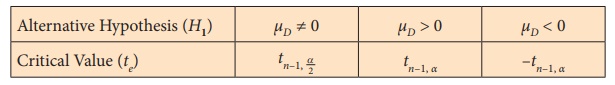
Step 7 : Decideon H₀ choosing the suitable rejection rule from the following table corresponding to H₁.

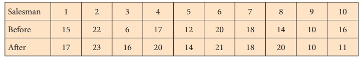
Example 2.5

A company gave an intensive training to its salesmen to increase the sales. A random sample of 10 salesmen was selected and the value (in lakhs of Rupees) of their sales per month, made before and after the training is recorded in the following table. Test whether there is any increase in mean sales at 5% level of significance.

Solution:

Step 1 : Hypotheses

Null Hypothesis H₀ : μ_D= 0

i.e., there is no significant increase in the mean sales after the training.

Alternative Hypothesis H₁ : μ_D> 0

i.e., there is significant increase in the mean sales after the training. It is a one-sided alternative hypothesis.

Step 2 : Data

Sample size n = 10

Step 3 : Level of significance

 α= 5%

Step 4 : Test statistic

Test statistic under the null hypothesis is

The sampling distribution of T under H₀ is t - distribution with (10–1) = 9 degrees of freedom.

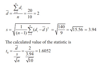
Step 5 : Calculation of test statistic

To find  and s:

Let x denote sales before training and y denote sales after training

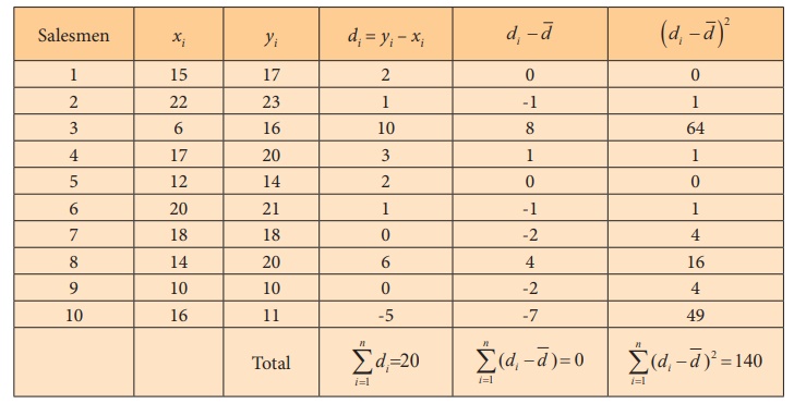
Here instead of d_i = x_i – y_i it is assumed d_i = y_i – x_i for calculations to be simpler.

Step 6 : Critical value

Since H₀ is a one-sided alternative hypothesis, the critical value at 5% level of significance is t_e = t_{n-1, α} =t_9,0.05 = 1.833

Step 7 : Decision

It is a one-tailed test. Since |t₀| = 1.6052 < t_e = t_{n-1, α} = t_9,0.05 = 1.833, H₀ is not rejected.

Hence, there is no evidence that the mean sales has increased after the training.