Applications in Heat Transfer & Fluid Mechanics

APPLICATIONS IN HEAT TRANSFER &FLUID MECHANICS

ONE DIMENSIONAL HEAT TRANSFER ELEMENT

In structural problem displacement at each nodel point is obtained. By using these displacement solutions, stresses and strains are calculated for each element. In structural problems, the unknowns are represented by the components of vector field. For example, in a two dimensional plate, the unknown quantity is the vector field u(x,y),where u is a (2x1)displacement vector.

Heat transfer can be defined as the transmission of energy from one region another region due to temperature difference. A knowledge of the temperature distribution within a body is important in many engineering problems. There are three modes of heat transfer.

They are:    (i) Conduction

(ii) Convection

(iii)Radiation

1Strong Form for Heat Conduction in One Dimension with Arbitrary Boundary Conditions

Following the same procedure as in Section, the portion of the boundary where the temperature is prescribed, i.e. the essential boundary is denoted by  T and the boundary where the flux is prescribed is recommended for  Science  and  Engineering  Track.  Denoted by q ;  these  are  the boundaries  with  natural  boundary  conditions. These  boundaries  are complementary, so

With the unit normal used in , we can express the natural boundary condition as qn ¼ q. For example, positive flux q causes heat inflow (negative q ) on the left boundary point where qn ¼ q ¼ q and heat outflow (positive q ) on the right boundary point where qn ¼ q ¼ q.

Strong form for 1D heat conduction problems

2Weak Form for Heat Conduction in One Dimension with Arbitrary Boundary Conditions

We again multiply the first two equations in the strong form by the weight function and integrate over the domains over which they hold, the domain for the differential equation and the domain q for the flux boundary condition, which

yields ws dx with w ¼

T and combining with gives

Recalling that w ¼ 0 on

Weak form for 1D heat conduction problems

Find T ðxÞ 2 U such that

Notice the similarity between

APPLICATION TO HEAT TRANSFER TWO-DIMENTIONAL

1Strong Form for Two-Point  Boundary Value Problems

The equations developed in this chapter for heat conduction, diffusion and elasticity problems are all of the following form:

Such one-dimensional problems are called two-point boundary value problems. gives the particular meanings of the above variables and parameters for several applications. The natural boundary conditions can also be generalized as (based on Becker et al. (1981))

Equation is a natural boundary condition because the derivative of the solution appears in it. reduces to the standard natural boundary conditions considered in the previous sections when bðx Þ ¼ 0. Notice that the essential boundary condition can be recovered as a limiting case of when bðxÞ is a penalty parameter, i.e. a large number In this case, and Equation is called a generalized boundary condition.

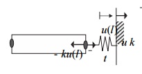
An example of the above generalized boundary condition is an elastic bar with a spring attached as shown in In this case, bðlÞ ¼ k and reduces to

where ¼ k is the spring constant. If the spring stiffness is set to a very large value, the above boundary condition enforces ¼ u; if we let k ¼ 0, the above boundary condition corresponds to a prescribed traction boundary. In practice, such generalized boundary conditions are often used to model the influence of the surroundings. For example, if the bar is a simplified model of a building and its foundation, the spring can represent the stiffness of the soil.

2 Two-Point Boundary Value Problem With Generalized Boundary Conditions

An example of the generalized boundary for elasticity problem.

Another example of the application of this boundary condition is convective heat transfer, where energy is transferred between the surface of the wall and the surrounding medium. Suppose convective heat transfer occurs at x ¼ l. Let T ðlÞ be the wall temperature at x ¼  l and T be the temperature in the  medium. Then the flux at the boundary x ¼  l is given by qð lÞ ¼  hðT ðlÞ T Þ, so  bðlÞ ¼  h and the boundary condition is    where h is convection coefficient, which has dimensions of W m 2  o C 1 . Note that when the convection coefficient is very large, the temperature T is immediately felt at x ¼ l and thus the essential boundary condition is again enforced as a limiting case of the natural boundary condition.

There are two approaches to deal with the boundary condition . We will call them the penalty and partition methods. In the penalty method, the essential boundary condition is enforced as a limiting case of the natural boundary condition by equating bðxÞ to a penalty parameter. The resulting strong form for the penalty method is given in.

General strong form for 1D problems-penalty method

þ f ¼  0   on          ;

In the partition approach, the total boundary is partitioned into the natural boundary, and the complementary essential boundary, The natural boundary condition has the generalized form defined by The resulting strong form for the partition method is summarized in.

3       Weak Form for Two-Point Boundary Value Problems

In this section, we will derive the general weak form for two-point boundary value problems. Both the penalty and partition methods described in will be considered. To obtain the general weak form for the penalty method, we multiply the two equations in the strong by the weight function and integrate over the domains over which they hold: the domain for the differential equation and the domain for the generalized boundary condition.

SCALE VARIABLE PROBLEM IN 2 DIMENSIONS

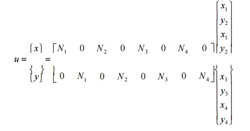
Ø Equation of Stiffness Matrix for 4 noded isoparametric quadrilateral element

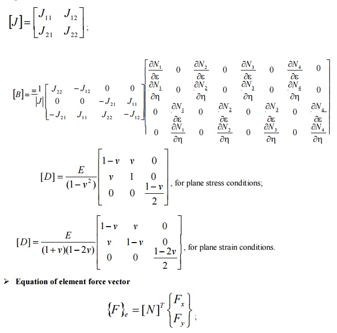
N –Shape function, 

F_x –load or force along x direction, 

F_y –load or force along y direction.

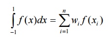
Ø Numerical Integration (Gaussian Quadrature)

The Gauss quadrature is one of the numerical integration methods to calculate the definite integrals. In FEA, this Gauss quadrature method is mostly preferred. In this method the numerical integration is achieved by the following expression,

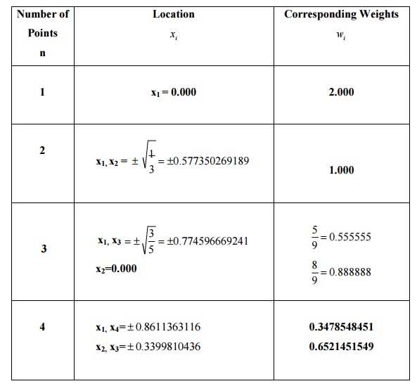
Table gives gauss points for integration from -1 to 1.

Ø Problem (I set)

1.     Evaluate 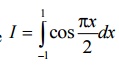 by applying 3 point Gaussian quadrature and compare with exact solution.

2.     2.  Evaluate 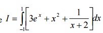  using one point and two point Gaussian quadrature. Compare with exact solution.

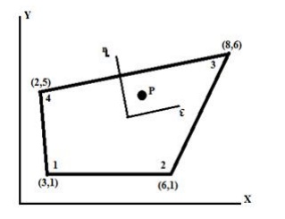
3.     3. For the isoparametric quadrilateral element shown in figure, determine the local co –ordinates of the point P which has Cartesian co-ordinates (7, 4).

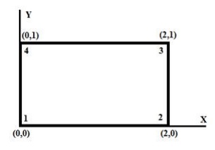
4.  A four noded rectangular element is in figure. Determine (i) Jacobian

matrix,  (ii)   Strain   – Displacement   matrix   and   (iii)   Element   Stresses.   Take

E=2x10⁵N/mm²,υ=        0.25,u=[0,0,0.003,0.004,0.006,.004,0,0]^T, Ɛ= 0, ɳ=0.

Assume plane stress condition.

2 DIMENTIONAL FLUID MECHANICS

The problem of linear elastostatics described in detail in can be extended to include the effects of inertia. The resulting equations of motion take the form

where u = u(x1 , x2, x3 , t) is the unknown displacement field, ρ is the mass density, and I = (0, T ) with T being a given ti me.  Also, u0 and v0 are the prescribed initi al displacement and  velocity  fields.  Clearly,  two  sets  of  boundary conditions  are  set  on  Γu   and  Γq  , respectively, and are assumed to hold throughout the time interval I . Likew ise, two sets of initial conditions are set for the whole domain Ω at time t = 0. The stron g form of the  resulting initial/boundary- value problem is stated as follows: given functions f , t, u¯ , u0 and v0, as well as a constitutive equation for σ, find u in Ω × I , such that the equations are satisfied.

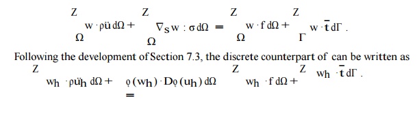
A Galerkin-based weak form of the linear elastostatics problem has been derived in Sec-tion In the elastodynamics case, the only substantial difference involves the inclusion of the term RΩ w • ρu¨ dΩ, as long as one adopts the semi-discrete approach.  As a result, the weak form at a fixed time can be expressed as  

Following a standard proced ure, the contribution of the forcing vector F^{i nt,e} due to interele- ment tractions is neglected upon assembly of the global equations . As a result, the equations is give rise to their assembled counterparts in the form

Mu  + Kuˆ =  F ,

where uˆ is the global unknown displacement vector¹ . The preceding equat ions are, of course, subject to initial conditions t hat can be written in vectorial form as uˆ(0) = uˆ₀ and vˆ(0) = vˆ₀

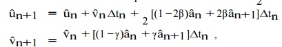
The most commonly emp loyed method for the numerical  solution of t he system of coupled linear second-order ordi nary differential equations is the Newmark m ethod.  This

method is based  on a time  series expansion of ˆu and ˆ   u˙ := v.ˆ  Concentrating on the time interval (tn ,tn+1], the New mark method is defined by the equations

It is clear that the Newmark equations  define a whole family of time inte grators.

It is important to distinguish this family into two categories, namely implicit and explicit integrators, corresponding to β > 0 and β = 0, respectively.

The overhead “hat” symbol is used to distinguish between the vector field u and the solution vector uˆemanating fr om the finite element approximation of the vector field u.

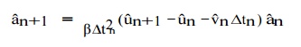
The general implicit Newmar k integration method may be implemented as follows: first, solve (9.18)₁ for aˆ_n+1 , namely write

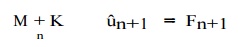
Then,  substitute (9.19) into the semi-discrete form (9.17) evaluated at tn+1  to find that

After solving for uˆ_n+1, one ma y compute the acceleration aˆ_n+1 from and the velocity vˆ_n+1 from.

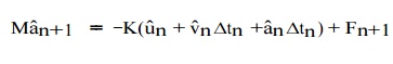
Finally, the general explicit N ewmark integration method may be implemented as follows: starting from the semi-discrete e quations evaluated at t_n+1, one may substitute uˆ_n+1from to find that

If M  is rendered  diagonal  (see discussion in our pages ), then aˆn+1 can  be determined without  solving any coupled  linear  algebraic  equations. Then,  ˆ are  the  velocities bvn+1 immediately computed  from (9. 18)2.  Also, the displacements uˆ n+1 are computed from indepen-dently of the acceleratio ns aˆn+1 .