2 Dimentional Fluid Mechanics

2 DIMENTIONAL FLUID MECHANICS

The problem of linear elastostatics described in detail in can be extended to include the effects of inertia. The resulting equations of motion take the form

where u = u(x1 , x2, x3 , t) is the unknown displacement field, ρ is the mass density, and I = (0, T ) with T being a given ti me.  Also, u0 and v0 are the prescribed initi al displacement and  velocity  fields.  Clearly,  two  sets  of  boundary conditions  are  set  on  Γu   and  Γq  , respectively, and are assumed to hold throughout the time interval I . Likew ise, two sets of initial conditions are set for the whole domain Ω at time t = 0. The stron g form of the  resulting initial/boundary- value problem is stated as follows: given functions f , t, u¯ , u0 and v0, as well as a constitutive equation for σ, find u in Ω × I , such that the equations are satisfied.

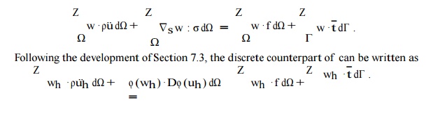
A Galerkin-based weak form of the linear elastostatics problem has been derived in Sec-tion In the elastodynamics case, the only substantial difference involves the inclusion of the term RΩ w • ρu¨ dΩ, as long as one adopts the semi-discrete approach.  As a result, the weak form at a fixed time can be expressed as  

Following a standard proced ure, the contribution of the forcing vector Fi nt,e due to interele- ment tractions is neglected upon assembly of the global equations . As a result, the equations is give rise to their assembled counterparts in the form

Mu  + Kuˆ =  F ,

where uˆ is the global unknown displacement vector1 . The preceding equat ions are, of course, subject to initial conditions t hat can be written in vectorial form as uˆ(0) = uˆ0 and vˆ(0) = vˆ0

The most commonly emp loyed method for the numerical  solution of t he system of coupled linear second-order ordi nary differential equations is the Newmark m ethod.  This

method is based  on a time  series expansion of ˆu and ˆ   u˙ := v.ˆ  Concentrating on the time interval (tn ,tn+1], the New mark method is defined by the equations

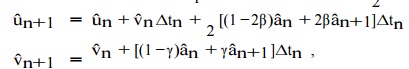
It is clear that the Newmark equations  define a whole family of time inte grators.

It is important to distinguish this family into two categories, namely implicit and explicit integrators, corresponding to β > 0 and β = 0, respectively.

The overhead “hat” symbol is used to distinguish between the vector field u and the solution vector uˆemanating fr om the finite element approximation of the vector field u.

The general implicit Newmar k integration method may be implemented as follows: first, solve (9.18)1 for aˆn+1 , namely write

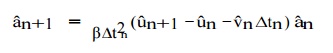
Then,  substitute (9.19) into the semi-discrete form (9.17) evaluated at tn+1  to find that

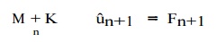
After solving for uˆn+1, one ma y compute the acceleration aˆn+1 from and the velocity vˆn+1 from.

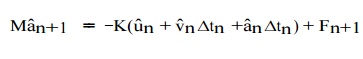
Finally, the general explicit N ewmark integration method may be implemented as follows: starting from the semi-discrete e quations evaluated at tn+1, one may substitute uˆn+1from to find that

If M  is rendered  diagonal  (see discussion in our pages ), then aˆn+1 can  be determined without  solving any coupled  linear  algebraic  equations. Then,  ˆ are  the  velocities bvn+1 immediately computed  from (9. 18)2.  Also, the displacements uˆ n+1 are computed from indepen-dently of the acceleratio ns aˆn+1 .