A Logical Representation of Data Flow

A Logical Representation of Data Flow

1 Introduction to Datalog

2 Datalog Rules

3 Intensional and Extensional Predicates

4 Execution of Datalog Programs

5 Incremental Evaluation of Datalog Programs

6 Problematic Datalog Rules

7 Exercises for Section 12.3

To this point, our representation of data-flow problems and solutions can be termed "set-theoretic." That is, we represent information as sets and compute results using operators like union and intersection. For instance, when we in-troduced the reaching-definitions problem in Section 9.2.4, we computed IN[B] and OUT[J3] for a block B, and we described these as sets of definitions. We represented the contents of the block B by its gen and kill sets.

To cope with the complexity of interprocedural analysis, we now introduce a more general and succinct notation based on logic. Instead of saying something like "definition D is in IN[ £ ?]," we shall use a notation like in(B,D) to mean the same thing. Doing so allows us to express succinct "rules" about inferring program facts. It also allows us to implement these rules efficiently, in a way that generalizes the bit-vector approach to set-theoretic operations. Finally, the logical approach allows us to combine what appear to be several indepen-dent analyses into one, integrated algorithm. For example, in Section 9.5 we described partial-redundancy elimination by a sequence of four data-flow anal-yses and two other intermediate steps. In the logical notation, all these steps could be combined into one collection of logical rules that are solved simulta-neously.

1. Introduction to Datalog

Catalog is a language that uses a Prolog-like notation, but whose semantics is far simpler than that of Prolog. To begin, the elements of Datalog are  atoms of  the  form p(X1,X2,... ,  Xn). Here,

1. p is a predicate — a symbol that represents a type of statement such as "a definition reaches the beginning of a block."

2. X1,X2,... ,Xn     are terms  such as  variables  or  constants.   We  shall  also allow simple expressions as arguments of a predicate.2

A ground atom is a predicate with only constants as arguments. Every ground atom asserts a particular fact, and its value is either true or false. It is often convenient to represent a predicate by a relation, or table of its true ground atoms. Each ground atom is represented by a single row, or tuple, of the relation. The columns of the relation are named by attributes, and each tuple has a component for each attribute. The attributes correspond to the components of the ground atoms represented by the relation. Any ground atom in the relation is true, and ground atoms not in the relation are false.

Example 1 2 . 1 1 : Let us suppose the predicate in(B,D) means "definition D reaches the beginning of block BP Then we might suppose that, for a particular flow graph, in{b1,d1) is true, as are in(b₂,di) and in(b2,d2). We might also suppose that for this flow graph, all other in facts are false. Then the relation in Fig. 12.12 represents the value of this predicate for this flow graph.

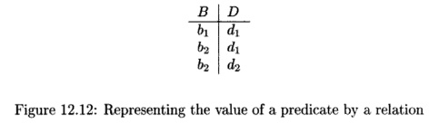
The attributes of the relation are B and D.  The three tuples of the relation are  (bi,di),  (b₂,di),  and  (b₂,d₂).

We shall also see at times an atom that is really a comparison between variables and constants. An example would be X ^ Y or X = 10. In these examples, the predicate is really the comparison operator. That is, we can think of X = 10 as if it were written in predicate form: equals(X, 10). There is an important difference between comparison predicates and others, however. A comparison predicate has its standard interpretation, while an ordinary pred-icate like in means only what it is defined to mean by a Datalog program (described next).

A literal is either an atom or a negated atom. We indicate negation with the word NOT in front of the atom. Thus, MOT in(B,D) is an assertion that definition D does not reach the beginning of block B.

2. Datalog Rules

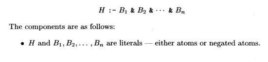
Rules are a way of expressing logical inferences. In Datalog, rules also serve to suggest how a computation of the true facts should be carried out. The form of a rule is

Datalog Conventions

We shall use the following conventions for Datalog programs:

1.                 Variables begin with a capital letter.

2.                 All other elements begin with lowercase letters or other symbols such as digits. These elements include predicates and constants that are arguments of predicates.

• H is the head and Bi,B2,..- ,Bn  form the body of the rule.

• Each of the IV s is sometimes called a subgoal of the rule.

We should read the : - symbol as "if." The meaning of a rule is "the head is true if the body is true." More precisely, we apply a rule to a given set of ground atoms as follows. Consider all possible substitutions of constants for the variables of the rule. If this substitution makes every subgoal of the body true (assuming that all and only the given ground atoms are true), then we can infer that the head with this substitution of constants for variables is a true fact. Substitutions that do not make all subgoals true give us no information; the head may or may not be true.

A Datalog program is a collection of rules. This program is applied to "data," that is, to a set of ground atoms for some of the predicates. The result of the program is the set of ground atoms inferred by applying the rules until no more inferences can be made.

Example 12 . 12 : A simple example of a Datalog program is the computation of paths in a graph, given its (directed) edges. That is, there is one predicate edge(X, Y) that means "there is an edge from node X to node Y." Another predicate path(X, Y) means that there is a path from X to Y. The rules defining paths are: 

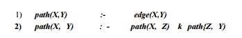
The first rule says that a single edge is a path. That is, whenever we replace variable X by a constant a and variable Y by a constant 6, and edge(a,b) is true (i.e., there is an edge from node a to node b), then path(a,b) is also true (i.e., there is a path from a to b). The second rule says that if there is a path from some node X to some node Z, and there is also a path from Z to node Y, then there is a path from X to Y. This rule expresses "transitive closure." Note that any path can be formed by taking the edges along the path and applying the transitive closure rule repeatedly.

For instance, suppose that the following facts (ground atoms) are true:

edge(l,2), edge(2,3), and edge(3,4). Then we can use the first rule with three different substitutions to infer path(l,2), path(2,3), and path(3,4). As an example, substituting X = 1 and Y = 2 instantiates the first rule to be path(l,2) : - edge(l,2). Since edge(l,2) is true, we infer path(l,2).

With these three path facts, we can use the second rule several times. If we substitute X = 1, Z = 2, and Y = 3, we instantiate the rule to be path(l,3) : - path(l,2) & path(2,3). Since both subgoals of the body have been inferred, they are known to be true, so we may infer the head: path(l,3).

Then, the substitution X = 1, Z = 3, and Y = 4 lets us infer the head path(l,4); that is, there is a path from node 1 to node 4.

3. Intensional and Extensional Predicates

It is conventional in Datalog programs to distinguish predicates as follows:

1. EDB, or extensional database, predicates are those that are defined a-priori. That is, their true facts are either given in a relation or table, or they are given by the meaning of the predicate (as would be the case for a comparison predicate, e.g.).

2. IDB, or  intensional database,  predicates are defined only by the rules.

A predicate must be IDB or EDB, and it can be only one of these. As a result, any predicate that appears in the head of one or more rules must be an IDB predicate. Predicates appearing in the body can be either IDB or EDB . For instance, in Example 12.12, edge is an EDB predicate and path is an IDB predicate. Recall that we were given some edge facts, such as edge(l,2), but the path facts were inferred by the rules.

When Datalog programs are used to express data-flow algorithms, the EDB predicates are computed from the flow graph itself. IDB predicates are then expressed by rules, and the data-flow problem is solved by inferring all possible IDB facts from the rules and the given EDB facts.

Example 12 . 13 : Let us consider how reaching definitions might be expressed in Datalog. First, it makes sense to think on a statement level, rather than a block level; that is, the construction of gen and kill sets from a basic block will be integrated with the computation of the reaching definitions themselves.

Thus, the block b1 suggested in Fig. 12.13 is typical. Notice that we identify points within the block numbered 0 , 1 , . . . , n, if n is the number of statements in the block. The ith definition is "at" point i, and there is no definition at point 0.

A point in the program must be represented by a pair (b,n), where 6 is a block name and n is an integer between 0 and the number of statements in block b. Our formulation requires two EDB predicates:

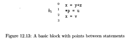
1. def(B, N, X) is true if and only if the iVth statement in block B may define variable X. For instance, in Fig. 12.13 def(bi,l,x) is true, def(bi,S,x) is true, and def(bi,2,Y) is true for every possible variable Y that p may point to at that point. For the moment, we shall assume that Y can be any variable of the type that p points to.

2. succ(B, N, C) is true if and only if block C is a successor of block B in the flow graph, and B has N statements. That is, control can flow from the point N of B to the point 0 of C. For instance, suppose that b2 is a predecessor of block b1 in Fig. 12.13, and b2 has 5 statements. Then succ(b2,5, &i) is true.

There is one IDB predicate, rd(B, N, C, M, X). It is intended to be true if and only if the definition of variable X at the M t h statement of block C reaches the point N in block B. The rules defining predicate rd are in Fig. 12.14.

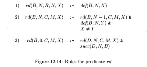
Rule (1) says that if the Nth statement of block B defines X, then that definition of X reaches the Nth point of B (i.e., the point immediately after the statement). This rule corresponds to the concept of "gen" in our earlier, set-theoretic formulation of reaching definitions.

Rule (2) represents the idea that a definition passes through a statement unless it is "killed," and the only way to kill a definition is to redefine its variable with 100% certainty. In detail, rule (2) says that the definition of variable X from the M t h statement of block C reaches the point N of block B if 

a) it reaches the previous point N — lot B, and

b) there is at least one variable Y, other than X, that may be defined at the TVth statement of B.

Finally, rule (3) expresses the flow of control in the graph. It says that the definition of X at the M t h statement of block C reaches the point 0 of B if there is some block D with TV statements, such that the definition of X reaches the end of D, and B is a successor of D. •

The EDB predicate succ from Example 12.13 clearly can be read off the flow graph. We can obtain deffrom the flow graph as well, if we are conservative and assume a pointer can point anywhere. If we want to limit the range of a pointer to variables of the appropriate type, then we can obtain type information from the symbol table, and use a smaller relation def. An option is to make def an IDB predicate and define it by rules. These rules will use more primitive EDB predicates, which can themselves be determined from the flow graph and symbol table.

Example 1 2 . 1 4 :  Suppose we introduce two new EDB predicates:

1. assign(B,N,X) is true  whenever  the iVth  statement of block  B  has  X on the left. Note that X can be a variable or a simple expression with an 1-value, like *p.   

2. type(X,T)  is true if the type of X  is T.  Again, X  can be any expression with an 1-value, and T can be any expression for a legal type.

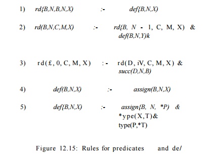
Then, we can write rules for  def,  making it an IDB predicate. Figure 12.15 is an expansion of Fig.  12.14, with two of the possible rules for def.  Rule (4) says that the TVth statement of block B defines X, if X is assigned by the TVth statement. Rule (5) says that X can also be defined by the iVth statement of block B if that statement assigns to * P , and X is any of the variables of the type that P points to. Other kinds of assignments would need other rules for def.

As an example of how we would make inferences using the rules of Fig. 12.15, let us re-examine the block bi of Fig. 12.13. The first statement assigns a value to variable x, so the fact assign(bi, 1,x) would be in the EDB . The third statement also assigns to x, so assign(bi,3, x) is another EDB fact. The second statement assigns indirectly through p, so a third EDB fact is assign(b_1: 2, *p). Rule (4) then allows us to infer def(bi,l,x) and def(bi,3,x).

Suppose that p is of type pointer-to-integer (*int), and x and y are integers. Then we may use rule (5), with B = h, N = 2, P = p, T - int, and X equal to either x or y, to infer def(b_1:2,x) and def(h,2,y). Similarly, we can infer the same about any other variable whose type is integer or coerceable to an integer.

4. Execution of Datalog Programs

Every set of Datalog rules defines relations for its IDB predicates, as a function of the relations that are given for its EDB predicates. Start with the assumption that th^ IDB relations are empty (i.e., the IDB predicates are false for all possible arguments). Then, repeatedly apply the rules, inferring new facts whenever the rules require us to do so. When the process converges, we are done, aijid the resulting IDB relations form the output of the program. This process is formalized in the next algorithm, which is similar to the iterative algorithms discussed in Chapter 9.

A l g o r i t h m 1 2 . 1 5 :  Simple evaluation of Datalog programs.

I N P U T : A Datalog program and sets of facts for each EDB predicate.

O U T P U T : Sets of facts for each IDB predicate.

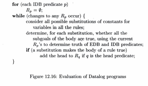
M E T H O D : For each predicate p in the program, let R_p be the relation of facts that are true for that predicate. If p is an EDB predicate, then R_p is the set of facts given for that predicate. If p is an IDB predicate, we shall compute R_p. Execute the algorithm in Fig. 12.16. •

Example 1 2 . 1 6 : The program in Example 12.12 computes paths in a graph. To apply Algorithm 12.15, we start with EDB predicate edge holding all the edges of the graph and with the relation for path empty. On the first round, rule (2) Vields nothing, since there are no path facts. But rule (1) causes all the edge facp to become path facts as well. That is, after the first round, we know path(a, 6) if and only if there is an edge from a to 6.

On the second round, rule (1) yields no new paths facts, because the EDB relation edge never changes. However, now rule (2) lets us put together two paths of length 1 to make paths of length 2. That is, after the second round, path(a, b) is true if and only if there is a path of length 1 or 2 from a to b. Similarly, on the third round, we can combine paths of length 2 or less to discover all paths of length 4 or less. On the fourth round, we discover paths of length up to to 8, and in general, after the ith round, path(a, b) is true if and only if there is a path from a to 6 of length 2l~1 or less.

5. Incremental Evaluation of Datalog Programs

There is an efficiency enhancement of Algorithm 12.15 possible. Observe that a new IDB fact can only be discovered on round i if it is the result of substituting constants in a rule, such that at least one of the subgoals becomes a fact that was just discovered on round i — The proof of that claim is that if all the facts among the subgoals were known at round i — 2, then the "new" fact would have been discovered when we made the same substitution of constants on round

To take advantage of this observation, introduce for each IDB predicate p a predicate newP that will hold only the newly discovered p-facts from the previous round. Each rule that has One or more IDB predicates among its subgoals is replaced by a collection of rules. Each rule in the collection is formed by replacing exactly one occurrence of some IDB predicate q in the body by newQ. Finally, for all rules, we replace the head predicate h by newH. The resulting rules are said to be in incremental form.

The relations for each IDB predicate p accumulates all the p-facts, as in Algorithm 12.15. In one round, we

1.  Apply the rules to evaluate the newP predicates.

Incremental Evaluation of Sets

It is also possible to solve set-theoretic data-flow problems incrementally. For example, in reaching definitions, a definition can only be newly discovered to be in m[B] on the 2th round if it was just discovered to be in OUT [ P ] for some predecessor P of B. The reason we do not generally try to solve such data-flow problems incrementally is that the bit-vector implementation of sets is so efficient. It is generally easier to fly through the complete vectors than to decide whether a fact is new or not.

2. Then, subtract p from newP, to make sure the facts in newP are truly new.

3.          Add the facts in newP to p.

4.          Set all the newX relations to 0 for the next round.

These ideas will be formalized in Algorithm 12.18. However, first, we shall give an example.

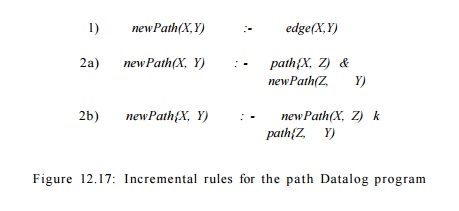
Example 1 2 . 1 7 : Consider the Datalog program in Example 12.12 again. The incremental form of the rules is given in Fig. 12.17. Rule (1) does not change, except in the head because it has no IDB subgoals in the body. However, rule (2), with two IDB subgoals, becomes two different rules. In each rule, one of the occurrences oipath in the body is replaced by newPath. Together, these rules enforce the idea that at least one of the two paths concatenated by the rule must have been discovered on the previous round.

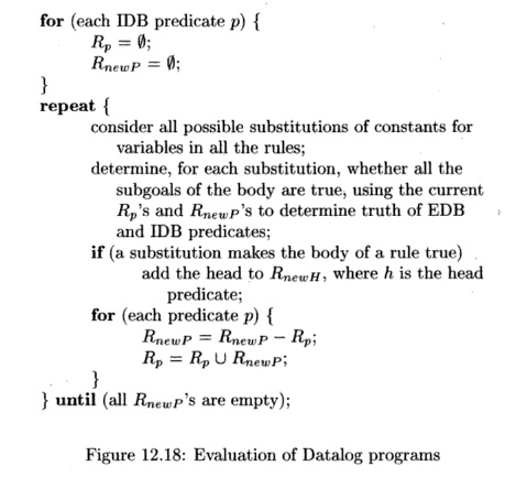
Algorithm 12.18 :         Incremental evaluation of Datalog programs.

INPUT : A Datalog program and sets of facts for each EDB predicate.

OUTPUT : Sets of facts for each IDB predicate.

METHOD : For each predicate p in the program, let Rp be the relation of facts that are true for that predicate. If p is an EDB predicate, then Rp is the set of facts given for that predicate. If p is an IDB predicate, we shall compute Rp. In addition, for each IDB predicate p, let Rnewp be a relation of "new" facts for predicate p.

1.         Modify the rules into the incremental form described above.

2.         Execute the algorithm in Fig. 12.18.

for (each IDB predicate p)  {

R_P    =  $;

RnewP — 0;

}

r e p e a t  {

consider all possible substitutions of constants for

variables in all the rules;

determine, for each substitution, whether all the

subgoals of the body are true, using the current

R_ps  and  R_newP^  to  determine  truth  of EDB

and IDB predicates;

if (a substitution makes the body of a rule true)

add the head to R_newH,  where h is the head

predicate;

for (each predicate p) {

RnewP — RnewP   Rp'i

Rp ⁼    Rp  U RnewP)

}

}  u n t i l (all Rnewp's are empty);

Figure 12.18:  Evaluation of Datalog programs

6. Problematic Datalog Rules

There are certain Datalog rules or programs that technically have no meaning and should not be used. The two most important risks are

1.          Unsafe rules: those that have a variable in the head that does not appear in the body in a way that constrains that variable to take on only values that appear in the EDB .

2.          Unstratified programs: sets of rules that have a recursion involving a nega-tion.

We shall elaborate on each of these risks.

Rule Safety

Any variable that appears in the head of a rule must also appear in the body. Moreover, that appearance must be in a subgoal that is an ordinary IDB or EDB atom. It is not acceptable if the variable appears only in a negated atom, or only in a comparison operator. The reason for this policy is to avoid rules that let us infer an infinite number of facts.

is unsafe for two reasons. Variable X appears only in the negated subgoal r(X) and the comparison X / Y. Y appears only in the comparison. The consequence is that p is true for an infinite number of pairs (X, Y), as long as r ( X ) is false and Y is anything other than X.

Stratified Datalog

In order for a program to make sense, recursion and negation must be separated. The formal requirement is as follows. We must be able to divide the IDB predicates into strata, so that if there is a rule with head predicate p and a subgoal of the form NOT #(•••), then q is either EDB or an IDB predicate in a lower stratum than p. As long as this rule is satisfied, we can evaluate the strata, lowest first, by Algorithm 12.15 or 12.18, and then treat the relations for the IDB predicates of that strata as if they were EDB for the computation of higher strata. However, if we violate this rule, then the iterative algorithm may fail to converge, as the next example shows.

Example 12.20 :  Consider the Datalog program consisting of the one rule:

Suppose e is an EDB predicate, and only e(l) is true.  Is p(l) true?

This program is not stratified. Whatever stratum we put p in, its rule has a subgoal that is negated and has an IDB predicate (namely p itself) that is surely not in a lower stratum than p.

If we apply the iterative algorithm, we start with R_p = 0, so initially, the answer is "no; p(l) is not true." However, the first iteration lets us infer p(l) , since both e(l) and NOT p(l) are true. But then the second iteration tells us p(l) is false. That is, substituting 1 for X in the rule does not allow us to infer p(l), since subgoal NOT p(l) is false. Similarly, the third iteration says p(l) is true, the fourth says it is false, and so on. We conclude that this unstratified program is meaningless, and do not consider it a valid program.

7. Exercises for Section 12.3

Exercise 1 2 . 3 . 1 : In this problem, we shall consider a reaching-definitions data-flow analysis that is simpler than that in Example 12.13. Assume that each statement by itself is a block, and initially assume that each statement defines exactly one variable.  The EDB predicate pred(I, J) means that statement I is a predecessor of statement J.  The EDB predicate defines (I, X) means that the variable defined by statement / is X. We shall use IDB predicates in(I, D) and out(I, D)  to mean that definition D reaches the beginning or end of statement  /, respectively. Note that a definition is really a statement number. Fig. 12.19 is a datalog program that expresses the usual algorithm for computing reaching definitions.

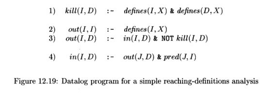
Notice that rule (1) says that a statement kills itself, but rule (2) assures that a statement is in its own "out set" anyway. Rule (3) is the normal transfer function, and rule (4) allows confluence, since I can have several predecessors.

Your problem is to modify the rules to handle the common case where a definition is ambiguous, e.g., an assignment through a pointer. In this situation, defines(I,X) may be true for several different X ' s and one I. A definition is best represented by a pair (D,X), where D is a statement, and X is one of the variables that may be defined at D. As a result, in and out become three- argument predicates; e.g., in(I, D,X) means that the (possible) definition of X at statement D reaches the beginning of statement I.

Exercise 1 2 . 3 . 2 : Write a Datalog program analogous to Fig. 12.19 to compute available expressions. In addition to predicate defines, use a predicate eval (I, X, O, Y) that says statement I causes expression XOY to be evaluated. Here, O is the operator in the expression, e.g., +.

Exercise 12 . 3 . 3: Write a Datalog program analogous to Fig. 12.19 to compute live variables. In addition to predicate defines, assume a predicate use(I, X) that says statement I uses variable X.

Exercise 12 . 3 . 4: In Section 9.5, we defined a data-flow calculation that in-volved six concepts: anticipated, available, earliest, postponable, latest, and used. Suppose we had written a Datalog program to define each of these in

terms of EDB concepts derivable from the program (e.g., gen and kill infor-mation) and others of these six concepts. Which of the six depend on which others? Which of these dependences are negated? Would the resulting Datalog program be stratified?

Exercise 12.3.5 : Suppose that the EDB predicate edge(X,Y) consists of the following facts:

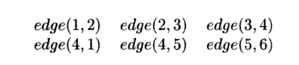
a)          Simulate the Datalog program of Example 12.12 on this data, using the simple evaluation strategy of Algorithm 12.15. Show the path facts dis-covered at each round.

b)          Simulate the Datalog program of Fig. 12.17 on this data, as part of the incremental evaluation strategy of Algorithm 12.18. Show the path facts discovered at each round.

Exercise 12.3.6 :  The following rule

is part of a larger Datalog program  P.

a)       Identify the head, body, and subgoals of this rule.

b)      Which predicates are certainly IDB predicates of program PI

c)       Which predicates are certainly EDB predicates of P?

d)          Is the rule safe?

e)           Is P stratified?

Exercise 12 . 3 . 7:  Convert the rules of Fig. 12.14 to incremental form.