Warshall’s and Floyd’s Algorithms

Warshall’s and Floyd’s Algorithms

In this section, we look at two well-known algorithms: Warshall’s algorithm for computing the transitive closure of a directed graph and Floyd’s algorithm for the all-pairs shortest-paths problem. These algorithms are based on essentially the same idea: exploit a relationship between a problem and its simpler rather than smaller version. Warshall and Floyd published their algorithms without mention-ing dynamic programming. Nevertheless, the algorithms certainly have a dynamic programming flavor and have come to be considered applications of this tech-nique.

Warshall’s Algorithm

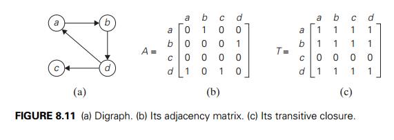
Recall that the adjacency matrix A = {aij } of a directed graph is the boolean matrix that has 1 in its ith row and j th column if and only if there is a directed edge from the ith vertex to the j th vertex. We may also be interested in a matrix containing the information about the existence of directed paths of arbitrary lengths between vertices of a given graph. Such a matrix, called the transitive closure of the digraph, would allow us to determine in constant time whether the j th vertex is reachable from the ith vertex.

Here are a few application examples. When a value in a spreadsheet cell is changed, the spreadsheet software must know all the other cells affected by the change. If the spreadsheet is modeled by a digraph whose vertices represent the spreadsheet cells and edges indicate cell dependencies, the transitive closure will provide such information. In software engineering, transitive closure can be used for investigating data flow and control flow dependencies as well as for inheritance testing of object-oriented software. In electronic engineering, it is used for redundancy identification and test generation for digital circuits.

DEFINITION The transitive closure of a directed graph with n vertices can be defined as the n × n boolean matrix T = {tij }, in which the element in the ith row and the j th column is 1 if there exists a nontrivial path (i.e., directed path of a positive length) from the ith vertex to the j th vertex; otherwise, tij is 0.

An example of a digraph, its adjacency matrix, and its transitive closure is given in Figure 8.11.

We can generate the transitive closure of a digraph with the help of depth-first search or breadth-first search. Performing either traversal starting at the ith

vertex gives the information about the vertices reachable from it and hence the columns that contain 1’s in the ith row of the transitive closure. Thus, doing such a traversal for every vertex as a starting point yields the transitive closure in its entirety.

Since this method traverses the same digraph several times, we should hope that a better algorithm can be found. Indeed, such an algorithm exists. It is called Warshall’s algorithm after Stephen Warshall, who discovered it [War62]. It is convenient to assume that the digraph’s vertices and hence the rows and columns of the adjacency matrix are numbered from 1 to n. Warshall’s algorithm constructs the transitive closure through a series of n × n boolean matrices:

Each of these matrices provides certain information about directed paths in the digraph. Specifically, the element rij(k) in the ith row and j th column of matrix R(k) (i, j = 1, 2, . . . , n, k = 0, 1, . . . , n) is equal to 1 if and only if there exists a directed path of a positive length from the ith vertex to the j th vertex with each intermediate vertex, if any, numbered not higher than k. Thus, the series starts with R(0), which does not allow any intermediate vertices in its paths; hence, R(0) is nothing other than the adjacency matrix of the digraph. (Recall that the adjacency matrix contains the information about one-edge paths, i.e., paths with no intermediate vertices.) R(1) contains the information about paths that can use the first vertex as intermediate; thus, with more freedom, so to speak, it may contain more 1’s than R(0). In general, each subsequent matrix in series (8.9) has one more vertex to use as intermediate for its paths than its predecessor and hence may, but does not have to, contain more 1’s. The last matrix in the series, R(n), reflects paths that can use all n vertices of the digraph as intermediate and hence is nothing other than the digraph’s transitive closure.

The central point of the algorithm is that we can compute all the elements of each matrix R(k) from its immediate predecessor R(k−1) in series (8.9). Let rij(k), the element in the ith row and j th column of matrix R(k), be equal to 1. This means that there exists a path from the ith vertex vi to the j th vertex vj with each intermediate vertex numbered not higher than k:

vi, a list of intermediate vertices each numbered not higher than k, vj .  (8.10)

Two situations regarding this path are possible. In the first, the list of its inter-mediate vertices does not contain the kth vertex. Then this path from vi to vj has

intermediate vertices numbered not higher than k − 1, and therefore rij(k−1) is equal to 1 as well. The second possibility is that path (8.10) does contain the kth vertex vk among the intermediate vertices. Without loss of generality, we may assume that vk occurs only once in that list. (If it is not the case, we can create a new path from vi to vj with this property by simply eliminating all the vertices between the first and last occurrences of vk in it.) With this caveat, path (8.10) can be rewritten as follows:

vi, vertices numbered ≤ k − 1, vk, vertices numbered ≤ k − 1, vj .

The first part of this representation means that there exists a path from vi to vk with each intermediate vertex numbered not higher than k − 1 (hence, rik(k−1) = 1), and the second part means that there exists a path from vk to vj with each intermediate vertex numbered not higher than k − 1 (hence, rkj(k−1) = 1).

What we have just proved is that if rij(k) = 1, then either rij(k−1) = 1 or both rik(k−1) = 1 and rkj(k−1) = 1. It is easy to see that the converse of this assertion is also

true. Thus, we have the following formula for generating the elements of matrix R(k) from the elements of matrix R(k−1):

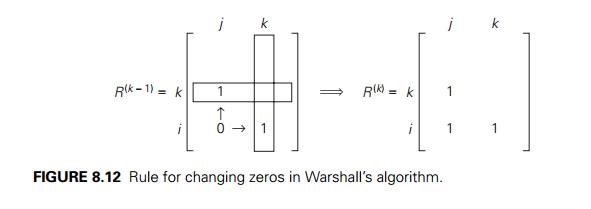
Formula (8.11) is at the heart of Warshall’s algorithm. This formula implies the following rule for generating elements of matrix R(k) from elements of matrix R(k−1), which is particularly convenient for applying Warshall’s algorithm by hand:

If an element rij is 1 in R(k−1), it remains 1 in R(k).

If an element rij is 0 in R(k−1), it has to be changed to 1 in R(k) if and only if the element in its row i and column k and the element in its column j and row

k are both 1’s in R(k−1). This rule is illustrated in Figure 8.12.

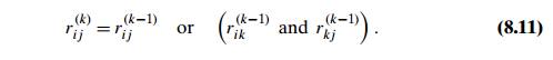
As an example, the application of Warshall’s algorithm to the digraph in Figure 8.11 is shown in Figure 8.13.

Here is pseudocode of Warshall’s algorithm.

ALGORITHM     Warshall(A[1..n, 1..n])

//Implements Warshall’s algorithm for computing the transitive closure //Input: The adjacency matrix A of a digraph with n vertices

//Output: The transitive closure of the digraph

R(0) ← A

for k ← 1 to n do for i ← 1 to n do

for j ← 1 to n do

R(k)[i, j ] ← R(k−1)[i, j ] or (R(k−1)[i, k] and R(k−1)[k, j ])

return R(n)

Several observations need to be made about Warshall’s algorithm. First, it is remarkably succinct, is it not? Still, its time efficiency is only  $(n3). In fact, for sparse graphs represented by their adjacency lists, the traversal-based algorithm

mentioned at the beginning of this section has a better asymptotic efficiency than Warshall’s algorithm (why?). We can speed up the above implementation of Warshall’s algorithm for some inputs by restructuring its innermost loop (see Problem 4 in this section’s exercises). Another way to make the algorithm run faster is to treat matrix rows as bit strings and employ the bitwise or operation available in most modern computer languages.

As to the space efficiency of Warshall’s algorithm, the situation is similar to that of computing a Fibonacci number and some other dynamic programming algorithms. Although we used separate matrices for recording intermediate results of the algorithm, this is, in fact, unnecessary. Problem 3 in this section’s exercises asks you to find a way of avoiding this wasteful use of the computer memory. Finally, we shall see below how the underlying idea of Warshall’s algorithm can be applied to the more general problem of finding lengths of shortest paths in weighted graphs.

Floyd’s Algorithm for the All-Pairs Shortest-Paths Problem

Given a weighted connected graph (undirected or directed), the all-pairs shortest-paths problem asks to find the distances—i.e., the lengths of the shortest paths— from each vertex to all other vertices. This is one of several variations of the problem involving shortest paths in graphs. Because of its important applications to communications, transportation networks, and operations research, it has been thoroughly studied over the years. Among recent applications of the all-pairs shortest-path problem is precomputing distances for motion planning in computer games.

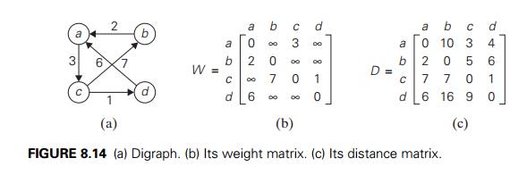
It is convenient to record the lengths of shortest paths in an n × n matrix D called the distance matrix: the element dij in the ith row and the j th column of this matrix indicates the length of the shortest path from the ith vertex to the j th vertex. For an example, see Figure 8.14.

We can generate the distance matrix with an algorithm that is very similar to Warshall’s algorithm. It is called Floyd’s algorithm after its co-inventor Robert W. Floyd.1 It is applicable to both undirected and directed weighted graphs provided that they do not contain a cycle of a negative length. (The distance between any two vertices in such a cycle can be made arbitrarily small by repeating the cycle enough times.) The algorithm can be enhanced to find not only the lengths of the shortest paths for all vertex pairs but also the shortest paths themselves (Problem 10 in this section’s exercises).

Floyd’s algorithm computes the distance matrix of a weighted graph with n vertices through a series of n × n matrices:

Each of these matrices contains the lengths of shortest paths with certain con-straints on the paths considered for the matrix in question. Specifically, the el-ement dij(k) in the ith row and the j th column of matrix D(k) (i, j = 1, 2, . . . , n, k = 0, 1, . . . , n) is equal to the length of the shortest path among all paths from the ith vertex to the j th vertex with each intermediate vertex, if any, numbered not higher than k. In particular, the series starts with D(0 ), which does not allow any intermediate vertices in its paths; hence, D(0) is simply the weight matrix of the graph. The last matrix in the series, D(n), contains the lengths of the shortest paths among all paths that can use all n vertices as intermediate and hence is nothing other than the distance matrix being sought.

As in Warshall’s algorithm, we can compute all the elements of each matrix D(k) from its immediate predecessor D(k−1) in series (8.12). Let dij(k) be the element in the ith row and the j th column of matrix D(k). This means that dij(k) is equal to the length of the shortest path among all paths from the ith vertex vi to the j th vertex vj with their intermediate vertices numbered not higher than k:

vi, a list of intermediate vertices each numbered not higher than k, vj .     (8.13)

We can partition all such paths into two disjoint subsets: those that do not use the kth vertex vk as intermediate and those that do. Since the paths of the first subset have their intermediate vertices numbered not higher than k − 1, the shortest of them is, by definition of our matrices, of length dij(k−1).

What is the length of the shortest path in the second subset? If the graph does not contain a cycle of a negative length, we can limit our attention only to the paths in the second subset that use vertex vk as their intermediate vertex exactly once (because visiting vk more than once can only increase the path’s length). All such paths have the following form:

vi, vertices numbered ≤ k − 1, vk, vertices numbered ≤ k − 1, vj .

In other words, each of the paths is made up of a path from vi to vk with each intermediate vertex numbered not higher than k − 1 and a path from vk to vj with each intermediate vertex numbered not higher than k − 1. The situation is depicted symbolically in Figure 8.15.

Since the length of the shortest path from vi to vk among the paths that use intermediate vertices numbered not higher than k − 1 is equal to dik(k−1) and the length of the shortest path from vk to vj among the paths that use intermediate

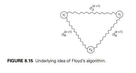
vertices numbered not higher than k − 1 is equal to dkj(k−1), the length of the shortest

path among the paths that use the kth vertex is equal to dik(k−1) + dkj(k−1). Taking into account the lengths of the shortest paths in both subsets leads to the following recurrence:

To put it another way, the element in row i and column j of the current distance matrix D(k−1) is replaced by the sum of the elements in the same row i and the column k and in the same column j and the row k if and only if the latter sum is smaller than its current value.

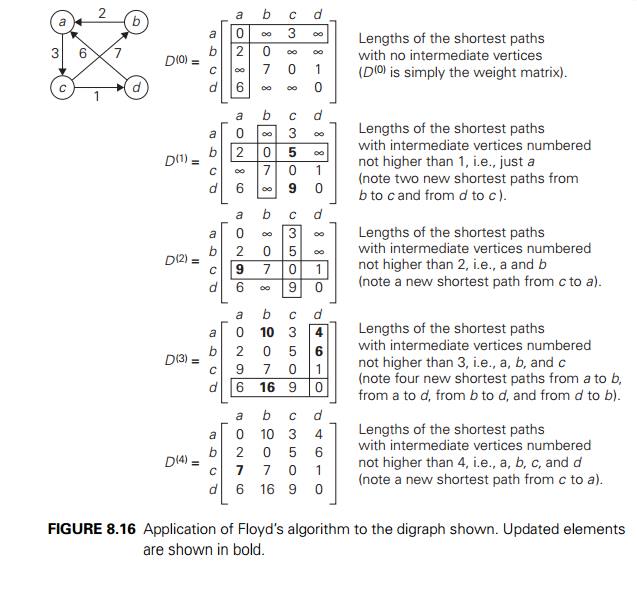
The application of Floyd’s algorithm to the graph in Figure 8.14 is illustrated in Figure 8.16.

Here is pseudocode of Floyd’s algorithm. It takes advantage of the fact that the next matrix in sequence (8.12) can be written over its predecessor.

ALGORITHM                 Floyd(W [1..n, 1..n])

//Implements Floyd’s algorithm for the all-pairs shortest-paths problem //Input: The weight matrix W of a graph with no negative-length cycle //Output: The distance matrix of the shortest paths’ lengths

D ← W //is not necessary if W can be overwritten for k ← 1 to n do

for i ← 1 to n do

for j ← 1 to n do

D[i, j ] ← min{D[i, j ], D[i, k] + D[k, j ]}

return D

Obviously, the time efficiency of Floyd’s algorithm is cubic—as is the time efficiency of Warshall’s algorithm. In the next chapter, we examine Dijkstra’s algorithm—another method for finding shortest paths.

Exercises 8.4

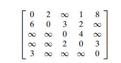
Apply Warshall’s algorithm to find the transitive closure of the digraph de-fined by the following adjacency matrix:

            a.  Prove that the time efficiency of Warshall’s algorithm is cubic.

Explain why the time efficiency class of Warshall’s algorithm is inferior to that of the traversal-based algorithm for sparse graphs represented by their adjacency lists.

            Explain how to implement Warshall’s algorithm without using extra memory for storing elements of the algorithm’s intermediate matrices.

            Explain how to restructure the innermost loop of the algorithm Warshall to make it run faster at least on some inputs.

            Rewrite pseudocode of Warshall’s algorithm assuming that the matrix rows are represented by bit strings on which the bitwise or operation can be per-formed.

            a. Explain how Warshall’s algorithm can be used to determine whether a given digraph is a dag (directed acyclic graph). Is it a good algorithm for this problem?

            Is it a good idea to apply Warshall’s algorithm to find the transitive closure of an undirected graph?

            Solve the all-pairs shortest-path problem for the digraph with the following

weight matrix:

            Prove that the next matrix in sequence (8.12) of Floyd’s algorithm can be written over its predecessor.

            Give an example of a graph or a digraph with negative weights for which Floyd’s algorithm does not yield the correct result.

            Enhance Floyd’s algorithm so that shortest paths themselves, not just their lengths, can be found.

Jack Straws In the game of Jack Straws, a number of plastic or wooden “straws” are dumped on the table and players try to remove them one by one without disturbing the other straws. Here, we are only concerned with whether various pairs of straws are connected by a path of touching straws. Given a list of the endpoints for n > 1 straws (as if they were dumped on a large piece of graph paper), determine all the pairs of straws that are connected. Note that touching is connecting, but also that two straws can be connected indirectly via other connected straws. [1994 East-Central Regionals of the ACM International Collegiate Programming Contest]

SUMMARY

Dynamic programming is a technique for solving problems with overlapping subproblems. Typically, these subproblems arise from a recurrence relating a solution to a given problem with solutions to its smaller subproblems of the same type. Dynamic programming suggests solving each smaller subproblem once and recording the results in a table from which a solution to the original problem can be then obtained.

Applicability of dynamic programming to an optimization problem requires the problem to satisfy the principle of optimality: an optimal solution to any of its instances must be made up of optimal solutions to its subinstances.

Among many other problems, the change-making problem with arbitrary coin denominations can be solved by dynamic programming.

Solving a knapsack problem by a dynamic programming algorithm exempli-fies an application of this technique to difficult problems of combinatorial optimization.

The memory function technique seeks to combine the strengths of the top-down and bottom-up approaches to solving problems with overlapping subproblems. It does this by solving, in the top-down fashion but only once, just the necessary subproblems of a given problem and recording their solutions in a table.

Dynamic programming can be used for constructing an optimal binary search tree for a given set of keys and known probabilities of searching for them.

Warshall’s algorithm for finding the transitive closure and Floyd’s algorithm for the all-pairs shortest-paths problem are based on the idea that can be interpreted as an application of the dynamic programming technique.