Greedy Technique

Chapter 9

Greedy Technique

Greed, for lack of a better word, is good! Greed is right! Greed works!

—Michael Douglas, US actor in the role of Gordon Gecko, in the film Wall Street, 1987

Let us revisit the change-making problem faced, at least subconsciously, by millions of cashiers all over the world: give change for a specific amount n with the least number of coins of the denominations d₁ > d₂ > ^{. . .} > d_m used in that locale. (Here, unlike Section 8.1, we assume that the denominations are ordered in decreasing order.) For example, the widely used coin denominations in the United States are d₁ = 25 (quarter), d₂ = 10 (dime), d₃ = 5 (nickel), and d₄ = 1 (penny). How would you give change with coins of these denominations of, say, 48 cents? If you came up with the answer 1 quarter, 2 dimes, and 3 pennies, you followed— consciously or not—a logical strategy of making a sequence of best choices among the currently available alternatives. Indeed, in the first step, you could have given one coin of any of the four denominations. “Greedy” thinking leads to giving one quarter because it reduces the remaining amount the most, namely, to 23 cents. In the second step, you had the same coins at your disposal, but you could not give a quarter, because it would have violated the problem’s constraints. So your best selection in this step was one dime, reducing the remaining amount to 13 cents.

Giving one more dime left you with 3 cents to be given with three pennies.

Is this solution to the instance of the change-making problem optimal? Yes, it is. In fact, one can prove that the greedy algorithm yields an optimal solution for every positive integer amount with these coin denominations. At the same time, it is easy to give an example of coin denominations that do not yield an optimal solution for some amounts—e.g., d₁ = 25, d₂ = 10, d₃ = 1 and n = 30.

The approach applied in the opening paragraph to the change-making prob-lem is called greedy. Computer scientists consider it a general design technique despite the fact that it is applicable to optimization problems only. The greedy approach suggests constructing a solution through a sequence of steps, each ex-panding a partially constructed solution obtained so far, until a complete solution to the problem is reached. On each step—and this is the central point of this technique—the choice made must be:

feasible, i.e., it has to satisfy the problem’s constraints

locally optimal, i.e., it has to be the best local choice among all feasible choices available on that step

irrevocable, i.e., once made, it cannot be changed on subsequent steps of the algorithm

These requirements explain the technique’s name: on each step, it suggests a “greedy” grab of the best alternative available in the hope that a sequence of locally optimal choices will yield a (globally) optimal solution to the entire problem. We refrain from a philosophical discussion of whether greed is good or bad. (If you have not seen the movie from which the chapter’s epigraph is taken, its hero did not end up well.) From our algorithmic perspective, the question is whether such a greedy strategy works or not. As we shall see, there are problems for which a sequence of locally optimal choices does yield an optimal solution for every instance of the problem in question. However, there are others for which this is not the case; for such problems, a greedy algorithm can still be of value if we are interested in or have to be satisfied with an approximate solution.

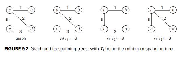
In the first two sections of the chapter, we discuss two classic algorithms for the minimum spanning tree problem: Prim’s algorithm and Kruskal’s algorithm. What is remarkable about these algorithms is the fact that they solve the same problem by applying the greedy approach in two different ways, and both of them always yield an optimal solution. In Section 9.3, we introduce another classic algorithm— Dijkstra’s algorithm for the shortest-path problem in a weighted graph. Section 9.4 is devoted to Huffman trees and their principal application, Huffman codes—an important data compression method that can be interpreted as an application of the greedy technique. Finally, a few examples of approximation algorithms based on the greedy approach are discussed in Section 12.3.

As a rule, greedy algorithms are both intuitively appealing and simple. Given an optimization problem, it is usually easy to figure out how to proceed in a greedy manner, possibly after considering a few small instances of the problem. What is usually more difficult is to prove that a greedy algorithm yields an optimal solution (when it does). One of the common ways to do this is illustrated by the proof given in Section 9.1: using mathematical induction, we show that a partially constructed solution obtained by the greedy algorithm on each iteration can be extended to an optimal solution to the problem.

The second way to prove optimality of a greedy algorithm is to show that on each step it does at least as well as any other algorithm could in advancing toward the problem’s goal. Consider, as an example, the following problem: find the minimum number of moves needed for a chess knight to go from one corner of a 100 × 100 board to the diagonally opposite corner. (The knight’s moves are L-shaped jumps: two squares horizontally or vertically followed by one square in the perpendicular direction.) A greedy solution is clear here: jump as close to the goal as possible on each move. Thus, if its start and finish squares are (1,1) and (100, 100), respectively, a sequence of 66 moves such as

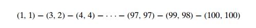
solves the problem. (The number k of two-move advances can be obtained from the equation 1 + 3k = 100.) Why is this a minimum-move solution? Because if we measure the distance to the goal by the Manhattan distance, which is the sum of the difference between the row numbers and the difference between the column numbers of two squares in question, the greedy algorithm decreases it by 3 on each move—the best the knight can do.

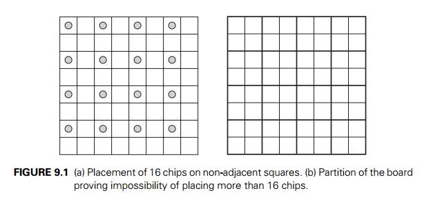
The third way is simply to show that the final result obtained by a greedy algorithm is optimal based on the algorithm’s output rather than the way it op-erates. As an example, consider the problem of placing the maximum number of chips on an 8 × 8 board so that no two chips are placed on the same or adjacent— vertically, horizontally, or diagonally—squares. To follow the prescription of the greedy strategy, we should place each new chip so as to leave as many available squares as possible for next chips. For example, starting with the upper left corner of the board, we will be able to place 16 chips as shown in Figure 9.1a. Why is this solution optimal? To see why, partition the board into sixteen 4 × 4 squares as shown in Figure 9.1b. Obviously, it is impossible to place more than one chip in each of these squares, which implies that the total number of nonadjacent chips on the board cannot exceed 16.

As a final comment, we should mention that a rather sophisticated theory has been developed behind the greedy technique, which is based on the abstract combinatorial structure called “matroid.” An interested reader can check such books as [Cor09] as well as a variety of Internet resources on the subject.