Prim’s Algorithm

Prim’s Algorithm

The following problem arises naturally in many practical situations: given n points, connect them in the cheapest possible way so that there will be a path between every pair of points. It has direct applications to the design of all kinds of networks— including communication, computer, transportation, and electrical—by providing the cheapest way to achieve connectivity. It identifies clusters of points in data sets. It has been used for classification purposes in archeology, biology, sociology, and other sciences. It is also helpful for constructing approximate solutions to more difficult problems such the traveling salesman problem (see Section 12.3).

We can represent the points given by vertices of a graph, possible connections by the graph’s edges, and the connection costs by the edge weights. Then the question can be posed as the minimum spanning tree problem, defined formally as follows.

DEFINITION A spanning tree of an undirected connected graph is its connected acyclic subgraph (i.e., a tree) that contains all the vertices of the graph. If such a graph has weights assigned to its edges, a minimum spanning tree is its spanning tree of the smallest weight, where the weight of a tree is defined as the sum of the weights on all its edges. The minimum spanning tree problem is the problem of finding a minimum spanning tree for a given weighted connected graph.

Figure 9.2 presents a simple example illustrating these notions.

If we were to try constructing a minimum spanning tree by exhaustive search, we would face two serious obstacles. First, the number of spanning trees grows exponentially with the graph size (at least for dense graphs). Second, generating all spanning trees for a given graph is not easy; in fact, it is more difficult than finding a minimum spanning tree for a weighted graph by using one of several efficient algorithms available for this problem. In this section, we outline Prim’s algorithm, which goes back to at least 1957¹ [Pri57].

Prim’s algorithm constructs a minimum spanning tree through a sequence of expanding subtrees. The initial subtree in such a sequence consists of a single vertex selected arbitrarily from the set V of the graph’s vertices. On each iteration, the algorithm expands the current tree in the greedy manner by simply attaching to it the nearest vertex not in that tree. (By the nearest vertex, we mean a vertex not in the tree connected to a vertex in the tree by an edge of the smallest weight. Ties can be broken arbitrarily.) The algorithm stops after all the graph’s vertices have been included in the tree being constructed. Since the algorithm expands a tree by exactly one vertex on each of its iterations, the total number of such iterations is n − 1, where n is the number of vertices in the graph. The tree generated by the algorithm is obtained as the set of edges used for the tree expansions.

Here is pseudocode of this algorithm.

ALGORITHM     Prim(G)

//Prim’s algorithm for constructing a minimum spanning tree //Input: A weighted connected graph G = V , E

//Output: E_T , the set of edges composing a minimum spanning tree of G V_T ← {v₀} //the set of tree vertices can be initialized with any vertex

E_T ← ∅

for i ← 1 to |V | − 1 do

find a minimum-weight edge e^∗ = (v^∗, u^∗) among all the edges (v, u) such that v is in V_T and u is in V − V_T

V_T ← V_T ∪ {u^∗} E_T ← E_T ∪ {e^∗}

return E_T

The nature of Prim’s algorithm makes it necessary to provide each vertex not in the current tree with the information about the shortest edge connecting the vertex to a tree vertex. We can provide such information by attaching two labels to a vertex: the name of the nearest tree vertex and the length (the weight) of the corresponding edge. Vertices that are not adjacent to any of the tree vertices can be given the ∞ label indicating their “infinite” distance to the tree vertices and a null label for the name of the nearest tree vertex. (Alternatively, we can split the vertices that are not in the tree into two sets, the “fringe” and the “unseen.” The fringe contains only the vertices that are not in the tree but are adjacent to at least one tree vertex. These are the candidates from which the next tree vertex is selected. The unseen vertices are all the other vertices of the graph, called “unseen” because they are yet to be affected by the algorithm.) With such labels, finding the next vertex to be added to the current tree T = ^*V_T , E_T ⁺ becomes a simple task of finding a vertex with the smallest distance label in the set V − V_T . Ties can be broken arbitrarily.

After we have identified a vertex u^∗ to be added to the tree, we need to perform two operations:

Move u^∗ from the set V − V_T to the set of tree vertices V_T .

For each remaining vertex u in V − V_T that is connected to u^∗ by a shorter edge than the u’s current distance label, update its labels by u^∗ and the weight of the edge between u^∗ and u, respectively.²

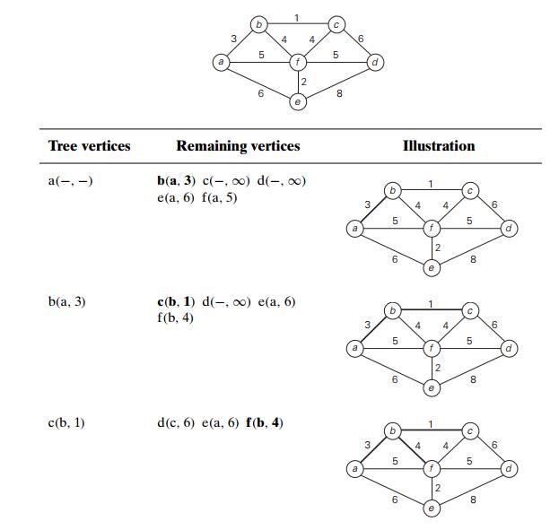
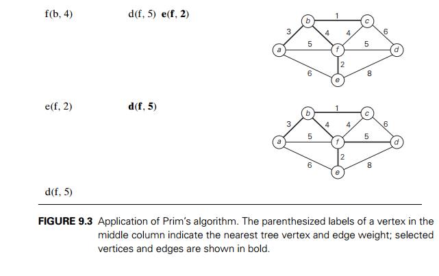
Figure 9.3 demonstrates the application of Prim’s algorithm to a specific graph. Does Prim’s algorithm always yield a minimum spanning tree? The answer to this question is yes. Let us prove by induction that each of the subtrees T_i,

i = 0, . . . , n − 1, generated by Prim’s algorithm is a part (i.e., a subgraph) of some minimum spanning tree. (This immediately implies, of course, that the last tree in the sequence, T_n−1, is a minimum spanning tree itself because it contains all n vertices of the graph.) The basis of the induction is trivial, since T₀ consists of a single vertex and hence must be a part of any minimum spanning tree. For the inductive step, let us assume that T_i−1 is part of some minimum spanning tree T . We need to prove that T_i, generated from T_i−1 by Prim’s algorithm, is also a part of a minimum spanning tree. We prove this by contradiction by assuming that no minimum spanning tree of the graph can contain T_i. Let e_i = (v, u) be the minimum weight edge from a vertex in T_i−1 to a vertex not in T_i−1 used by Prim’s algorithm to expand T_i−1 to T_i. 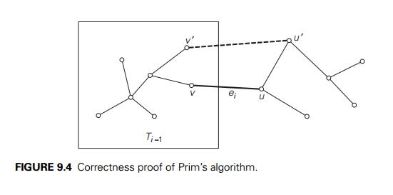By our assumption, e_i cannot belong to any minimum spanning tree, including T . Therefore, if we add e_i to T , a cycle must be formed (Figure 9.4).

In addition to edge e_i = (v, u), this cycle must contain another edge (v , u ) connecting a vertex v ∈ T_i−1 to a vertex u that is not in T_i−1. (It is possible that v coincides with v or u coincides with u but not both.) If we now delete the edge (v , u ) from this cycle, we will obtain another spanning tree of the entire graph whose weight is less than or equal to the weight of T since the weight of e_i is less than or equal to the weight of (v , u ). Hence, this spanning tree is a minimum spanning tree, which contradicts the assumption that no minimum spanning tree contains T_i. This completes the correctness proof of Prim’s algorithm.

How efficient is Prim’s algorithm? The answer depends on the data structures chosen for the graph itself and for the priority queue of the set V − V_T whose vertex priorities are the distances to the nearest tree vertices. (You may want to take another look at the example in Figure 9.3 to see that the set V − V_T indeed operates as a priority queue.) In particular, if a graph is represented by its weight matrix and the priority queue is implemented as an unordered array, the algorithm’s running time will be in  (|V |²). Indeed, on each of the |V | − 1 iterations, the array implementing the priority queue is traversed to find and delete the minimum and then to update, if necessary, the priorities of the remaining vertices.

We can also implement the priority queue as a min-heap. A min-heap is a mirror image of the heap structure discussed in Section 6.4. (In fact, it can be im-plemented by constructing a heap after negating all the key values given.) Namely, a min-heap is a complete binary tree in which every element is less than or equal

to its children. All the principal properties of heaps remain valid for min-heaps, with some obvious modifications. For example, the root of a min-heap contains the smallest rather than the largest element. Deletion of the smallest element from and insertion of a new element into a min-heap of size n are O(log n) operations, and so is the operation of changing an element’s priority (see Problem 15 in this section’s exercises).

If a graph is represented by its adjacency lists and the priority queue is im-plemented as a min-heap, the running time of the algorithm is in O(|E| log |V |). This is because the algorithm performs |V | − 1 deletions of the smallest element and makes |E| verifications and, possibly, changes of an element’s priority in a min-heap of size not exceeding |V |. Each of these operations, as noted earlier, is a O(log |V |) operation. Hence, the running time of this implementation of Prim’s algorithm is in

because, in a connected graph, |V | − 1 ≤ |E|.

In the next section, you will find another greedy algorithm for the minimum spanning tree problem, which is “greedy” in a manner different from that of Prim’s algorithm.

Exercises 9.1

            Write pseudocode of the greedy algorithm for the change-making problem, with an amount n and coin denominations d₁ > d₂ > ^{. . .} > d_m as its input. What is the time efficiency class of your algorithm?

            Design a greedy algorithm for the assignment problem (see Section 3.4). Does your greedy algorithm always yield an optimal solution?

Job scheduling Consider the problem of scheduling n jobs of known dura-tions t₁, t₂, . . . , t_n for execution by a single processor. The jobs can be executed in any order, one job at a time. You want to find a schedule that minimizes the total time spent by all the jobs in the system. (The time spent by one job in the system is the sum of the time spent by this job in waiting plus the time spent on its execution.)

Design a greedy algorithm for this problem. Does the greedy algorithm always yield an optimal solution?

         Compatible intervals Given n open intervals (a₁, b₁), (a₂, b₂), . . . , (a_n, b_n) on the real line, each representing start and end times of some activity requiring the same resource, the task is to find the largest number of these intervals so that no two of them overlap. Investigate the three greedy algorithms based on

            earliest start first.

            shortest duration first.

            earliest finish first.

For each of the three algorithms, either prove that the algorithm always yields an optimal solution or give a counterexample showing this not to be the case.

         Bridge crossing revisited Consider the generalization of the bridge crossing puzzle (Problem 2 in Exercises 1.2) in which we have n > 1 people whose bridge crossing times are t₁, t₂, . . . , t_n. All the other conditions of the problem remain the same: at most two people at a time can cross the bridge (and they move with the speed of the slower of the two) and they must carry with them the only flashlight the group has.

Design a greedy algorithm for this problem and find how long it will take to cross the bridge by using this algorithm. Does your algorithm yield a minimum crossing time for every instance of the problem? If it does—prove it; if it does not—find an instance with the smallest number of people for which this happens.

         Averaging down There are n > 1 identical vessels, one of them with W pints of water and the others empty. You are allowed to perform the following operation: take two of the vessels and split the total amount of water in them equally between them. The object is to achieve a minimum amount of water in the vessel containing all the water in the initial set up by a sequence of such operations. What is the best way to do this?

         Rumor spreading There are n people, each in possession of a different rumor. They want to share all the rumors with each other by sending electronic messages. Assume that a sender includes all the rumors he or she knows at the time the message is sent and that a message may only have one addressee.

Design a greedy algorithm that always yields the minimum number of messages they need to send to guarantee that every one of them gets all the rumors.

         Bachet’s problem of weights Find an optimal set of n weights {w₁, w₂, . . . , w_n} so that it would be possible to weigh on a balance scale any integer load in the largest possible range from 1 to W , provided

  weights can be put only on the free cup of the scale. weights can be put on both cups of the scale.

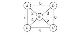
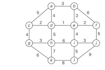
a. Apply Prim’s algorithm to the following graph. Include in the priority queue all the vertices not already in the tree.

Apply Prim’s algorithm to the following graph. Include in the priority queue only the fringe vertices (the vertices not in the current tree which are adjacent to at least one tree vertex).

            The notion of a minimum spanning tree is applicable to a connected weighted graph. Do we have to check a graph’s connectivity before applying Prim’s algorithm, or can the algorithm do it by itself?

            Does Prim’s algorithm always work correctly on graphs with negative edge weights?

            Let T be a minimum spanning tree of graph G obtained by Prim’s algorithm. Let G_new be a graph obtained by adding to G a new vertex and some edges, with weights, connecting the new vertex to some vertices in G. Can we con-struct a minimum spanning tree of G_new by adding one of the new edges to T ? If you answer yes, explain how; if you answer no, explain why not.

            How can one use Prim’s algorithm to find a spanning tree of a connected graph with no weights on its edges? Is it a good algorithm for this problem?

            Prove that any weighted connected graph with distinct weights has exactly one minimum spanning tree.

Outline an efficient algorithm for changing an element’s value in a min-heap. What is the time efficiency of your algorithm?