Chapter: Introduction to the Design and Analysis of Algorithms : Greedy Technique
KruskalŌĆÖs Algorithm
KruskalŌĆÖs Algorithm
In the previous section, we
considered the greedy algorithm that ŌĆ£growsŌĆØ a mini-mum spanning tree through a
greedy inclusion of the nearest vertex to the vertices already in the tree.
Remarkably, there is another greedy algorithm for the mini-mum spanning tree
problem that also always yields an optimal solution. It is named KruskalŌĆÖs
algorithm after Joseph Kruskal, who discovered this algorithm when he
was a second-year graduate student [Kru56]. KruskalŌĆÖs algorithm looks at a
minimum spanning tree of a weighted connected graph G = V
, E as an acyclic subgraph with |V | ŌłÆ 1 edges for which the sum of the edge weights
is the smallest. (It is not difficult to prove that such a subgraph must be a
tree.) Consequently, the algorithm constructs a minimum spanning tree as an
expanding sequence of subgraphs that are always acyclic but are not necessarily
connected on the inter-mediate stages of the algorithm.
The algorithm begins by
sorting the graphŌĆÖs edges in nondecreasing order of their weights. Then,
starting with the empty subgraph, it scans this sorted list, adding the next
edge on the list to the current subgraph if such an inclusion does not create a
cycle and simply skipping the edge otherwise.
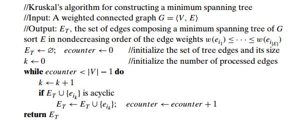
ALGORITHM Kruskal(G)
//KruskalŌĆÖs algorithm for
constructing a minimum spanning tree //Input: A weighted connected graph G = V
, E
//Output: ET , the set of edges composing a
minimum spanning tree of G sort E in nondecreasing order of the edge weights w(ei1) Ōēż . . . Ōēż w(ei|E| )
The correctness of KruskalŌĆÖs
algorithm can be proved by repeating the essen-tial steps of the proof of
PrimŌĆÖs algorithm given in the previous section. The fact that ET is actually a tree in PrimŌĆÖs algorithm but
generally just an acyclic subgraph in KruskalŌĆÖs algorithm turns out to be an
obstacle that can be overcome.
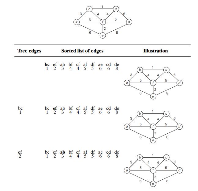
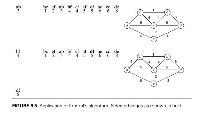
Figure 9.5 demonstrates the
application of KruskalŌĆÖs algorithm to the same graph we used for illustrating
PrimŌĆÖs algorithm in Section 9.1. As you trace the algorithmŌĆÖs operations, note
the disconnectedness of some of the intermediate subgraphs.
Applying PrimŌĆÖs and KruskalŌĆÖs
algorithms to the same small graph by hand may create the impression that the
latter is simpler than the former. This impres-sion is wrong because, on each
of its iterations, KruskalŌĆÖs algorithm has to check whether the addition of the
next edge to the edges already selected would create a
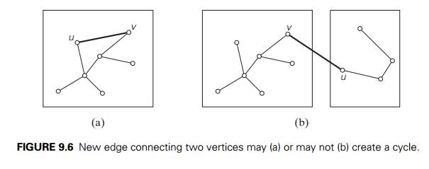
cycle. It is not difficult to
see that a new cycle is created if and only if the new edge connects two
vertices already connected by a path, i.e., if and only if the two ver-tices
belong to the same connected component (Figure 9.6). Note also that each
connected component of a subgraph generated by KruskalŌĆÖs algorithm is a tree
because it has no cycles.
In view of these
observations, it is convenient to use a slightly different interpretation of
KruskalŌĆÖs algorithm. We can consider the algorithmŌĆÖs operations as a
progression through a series of forests containing all the vertices of a given graph and some of its edges. The initial forest consists of |V | trivial trees, each comprising a single vertex
of the graph. The final forest consists of a single tree, which is a minimum
spanning tree of the graph. On each iteration, the algorithm takes the next
edge (u, v) from the sorted list of the
graphŌĆÖs edges, finds the trees containing the vertices u and v, and, if these trees are not the same, unites
them in a larger tree by adding the edge (u, v).
Fortunately, there are
efficient algorithms for doing so, including the crucial check for whether two
vertices belong to the same tree. They are called union-find algorithms. We
discuss them in the following subsection. With an efficient union-find algorithm,
the running time of KruskalŌĆÖs algorithm will be dominated by the time needed
for sorting the edge weights of a given graph. Hence, with an efficient sorting
algorithm, the time efficiency of KruskalŌĆÖs algorithm will be in
O(|E| log |E|).
Disjoint
Subsets and Union-Find Algorithms
KruskalŌĆÖs algorithm is one of
a number of applications that require a dynamic partition of some n element set S into a collection of disjoint subsets S1, S2, . . . , Sk. After being initialized as a collection of n one-element subsets, each containing a
different element of S, the collection is subjected
to a sequence of intermixed union and find operations. (Note that the number of
union operations in any such sequence must be bounded above by n ŌłÆ 1 because each union increases a subsetŌĆÖs size
at least by 1 and there are only n elements in the entire set S.) Thus, we are dealing here with an abstract
data type of a collection of disjoint subsets of a finite set with the following
operations:
makeset(x) creates a one-element set {x}. It is assumed that this operation can be applied to each of the elements of
set S only once.
find(x) returns a subset containing x.
union(x,
y) constructs the union of the disjoint subsets Sx and Sy containing x and
y, respectively, and adds it to the collection to replace Sx and Sy, which are deleted from it.
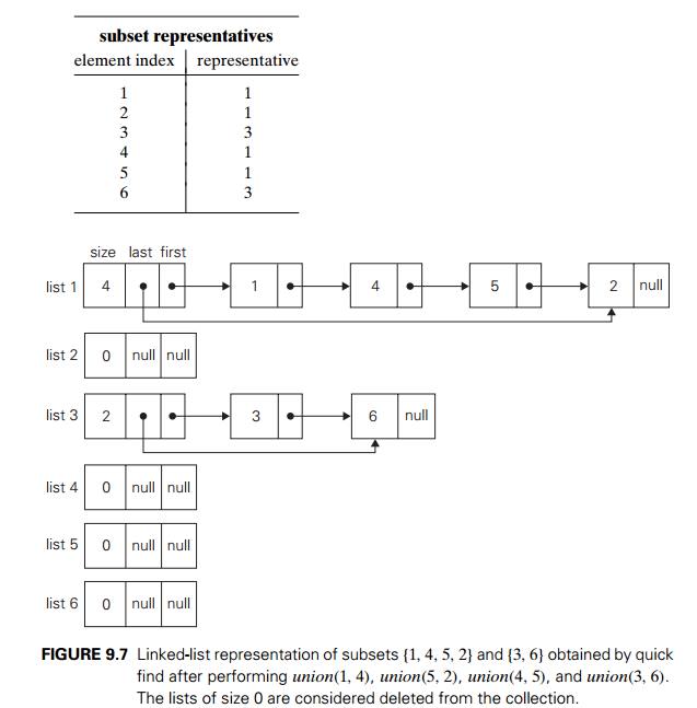
For example, let S = {1, 2, 3, 4, 5, 6}. Then makeset(i) creates the set {i} and applying this operation six times
initializes the structure to the collection of six singleton sets:
{1}, {2}, {3}, {4}, {5}, {6}.
Performing union(1, 4) and union(5, 2) yields
{1, 4}, {5, 2}, {3}, {6},
and, if followed by union(4, 5) and then by union(3, 6), we end up with the disjoint
subsets
{1, 4, 5, 2}, {3, 6}.
Most implementations of this
abstract data type use one element from each of the disjoint subsets in a
collection as that subsetŌĆÖs representative. Some
implemen-tations do not impose any specific constraints on such a
representative; others do so by requiring, say, the smallest element of each
subset to be used as the subsetŌĆÖs representative. Also, it is usually assumed
that set elements are (or can be mapped into) integers.
There are two principal
alternatives for implementing this data structure. The first one, called the quick
find, optimizes the time efficiency of the find operation; the second
one, called the quick union, optimizes the union operation.
The quick find uses an array
indexed by the elements of the underlying set S; the arrayŌĆÖs values indicate the
representatives of the subsets containing those elements. Each subset is implemented as a
linked list whose header contains the pointers to the first and last elements
of the list along with the number of elements in the list (see Figure 9.7 for
an example).
Under this scheme, the
implementation of makeset(x) requires assigning the corresponding element
in the representative array to x and initializing the
corre-sponding linked list to a single node with the x value. The time efficiency of this operation
is obviously in (1), and hence the initialization
of n singleton subsets is in (n). The efficiency of find(x) is also in (1): all we need to do is to retrieve the xŌĆÖs representative in the representative array.
Executing union(x,
y) takes longer. A straightforward solution
would simply append the yŌĆÖs list to the end of the xŌĆÖs list, update the information about their
representative for all the elements in the
y list, and then delete the yŌĆÖs list from the collection. It is easy to
verify, however, that with this algorithm the
sequence of union operations
union(2, 1), union(3, 2), . . . , union(i + 1, i), . . . , union(n,
n ŌłÆ 1)
runs in (n2) time, which is slow compared with several
known alternatives.
A simple way to improve the
overall efficiency of a sequence of union oper-ations is to always append the
shorter of the two lists to the longer one, with ties broken arbitrarily. Of
course, the size of each list is assumed to be available by, say, storing the
number of elements in the listŌĆÖs header. This modification is called the
union by size. Though it does not improve
the worst-case efficiency of a single ap-plication of the union operation (it
is still in (n)), the worst-case running time of any
legitimate sequence of union-by-size operations turns out to be in O(n log n).3 Here is a proof of this assertion. Let ai be an element of set S whose disjoint subsets we manipulate, and let Ai be the number of times aiŌĆÖs representative is updated in a sequence of
union-by-size operations. How large
can Ai get if set S has n elements? Each time aiŌĆÖs representative is updated, ai must be in a smaller subset involved in
computing the union whose size will be at least twice as large as the size of
the subset containing ai. Hence, when aiŌĆÖs representative is updated for the first
time, the resulting set will have at least two elements; when it is updated for
the second time, the resulting set will have at least four elements; and, in
general, if it is updated Ai times, the resulting set will have at least 2Ai
elements. Since the entire set S has n elements, 2Ai Ōēż n and hence Ai Ōēż log2 n. Therefore, the total number
of possible updates of the representatives for all n elements in S
will not exceed n log2 n.
Thus, for union by size, the
time efficiency of a sequence of at most n ŌłÆ 1 unions and m finds is in O(n log n + m).
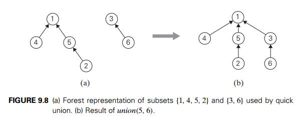
The quick unionŌĆöthe second
principal alternative for implementing disjoint subsetsŌĆörepresents each subset
by a rooted tree. The nodes of the tree contain the subsetŌĆÖs elements (one per
node), with the rootŌĆÖs element considered the subsetŌĆÖs representative; the
treeŌĆÖs edges are directed from children to their parents (Figure 9.8). In
addition, a mapping of the set elements to their tree nodesŌĆö implemented, say,
as an array of pointersŌĆöis maintained. This mapping is not shown in Figure 9.8
for the sake of simplicity.
For this implementation, makeset(x) requires the creation of a single-node tree,
which is a (1) operation; hence, the
initialization of n singleton subsets is in (n). A union(x, y) is implemented by attaching the root of the yŌĆÖs tree to the root of the xŌĆÖs tree (and deleting the yŌĆÖs tree from the collection by making the
pointer to its root null). The time efficiency of this operation is clearly (1). A find(x) is
performed by following the
pointer chain from the node containing x to the treeŌĆÖs root whose element is returned
as the subsetŌĆÖs representative. Accordingly, the time efficiency of a single
find operation is in O(n) because a tree representing
a subset can degenerate into a linked list with n nodes.
This time bound can be
improved. The straightforward way for doing so is to always perform a union
operation by attaching a smaller tree to the root of a larger one, with ties
broken arbitrarily. The size of a tree can be measured either by the number of
nodes (this version is called union by size) or by its height
(this version is called union by rank). Of course, these
options require storing, for each node of the tree, either the number of node
descendants or the height of the subtree rooted at that node, respectively. One
can easily prove that in either case the height of the tree will be logarithmic,
making it possible to execute each find in O(log n) time. Thus, for quick union,
the time efficiency of a sequence of at most n ŌłÆ 1 unions and m finds is in O(n + m log n).
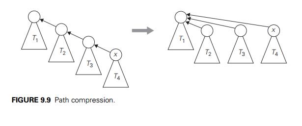
In fact, an even better
efficiency can be obtained by combining either vari-ety of quick union with path
compression. This modification makes every node encountered during the
execution of a find operation point to the treeŌĆÖs root (Fig-ure 9.9). According
to a quite sophisticated analysis that goes beyond the level of this book (see
[Tar84]), this and similar techniques improve the efficiency of a sequence of
at most n ŌłÆ 1 unions and m finds to only slightly worse than linear.
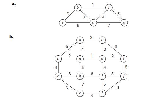
Exercises 9.2
Apply KruskalŌĆÖs algorithm to
find a minimum spanning tree of the following graphs.
Indicate whether the following statements are true or false:
If e is a minimum-weight edge in
a connected weighted graph, it must be among edges of at least one minimum
spanning tree of the graph.
If e is a minimum-weight edge in
a connected weighted graph, it must be among edges of each minimum spanning
tree of the graph.
If edge weights of a connected weighted graph are all distinct, the
graph must have exactly one minimum spanning tree.
If edge weights of a connected weighted graph are not all distinct,
the graph must have more than one minimum spanning tree.
What changes, if any, need to be made in algorithm Kruskal to make it find a minimum
spanning forest for an arbitrary graph? (A minimum spanning forest is a
forest whose trees are minimum spanning trees of the graphŌĆÖs connected
components.)
Does KruskalŌĆÖs algorithm work correctly on graphs that have
negative edge weights?
Design an algorithm for finding a maximum spanning treeŌĆöa
spanning tree with the largest possible edge weightŌĆöof a weighted connected
graph.
Rewrite pseudocode of KruskalŌĆÖs algorithm in terms of the
operations of the disjoint subsetsŌĆÖ ADT.
Prove the correctness of KruskalŌĆÖs algorithm.
Prove that the time efficiency of find(x) is in O(log n) for the union-by-size
version of quick union.
Find at least two Web sites with animations of KruskalŌĆÖs and PrimŌĆÖs
algorithms. Discuss their merits and demerits.
Design and conduct an experiment to empirically compare the
efficiencies of PrimŌĆÖs and KruskalŌĆÖs algorithms on random graphs of different
sizes and densities.
Steiner tree Four villages are located at
the vertices of a unit square in the Euclidean
plane. You are asked to connect them by the shortest network of roads so that
there is a path between every pair of the villages along those roads. Find such
a network.
Write a program generating a random maze based on
PrimŌĆÖs algorithm.
KruskalŌĆÖs algorithm.
Related Topics