Unconstrained Problems -Classical Optimization Theory

UNCONSTRAINED PROBLEMS

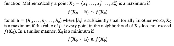
An extreme point of a function f(X) defines either a maximum or a minimum of the

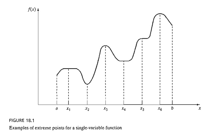
Figure 18.1 illustrates the maxima and minima of a single-variable function f(x) over the interval [a,b]. The points x₁, x₂, x₃, x₄, and x₆ are all extrema of f(x), with x_l, x₃, and x₆ as maxima and x₂ and x₄ as minima. Because

f(x₆) is a global or absolute maximum, and f(x₁) and f(x₃) are local or relative maxima. Similarly,f(x₄) is a local minimum and f(x₂) is a global minimum.

Although x₁ (in Figure 18.1) is a maximum point, it differs from remaining local maxima in that the value of f corresponding to at least one point in the neighborhood of x₁ equals f(x₁) In this respect, x₁ is a weak maximum, whereas x₃ and x₆ are strong maxima. In general, for h as defined earlier, X _o is a weak maximum if f(X _o + h) ≤ f(X ₀) and a strong maximum if f(X _o + h) < f(X _o).

In Figure 18.1, the first derivative (slope) of f equals zero at all extrema. However, this property is also satisfied at inflection and saddle points, such as x₅. If a point with zero slope (gradient) is not an extremum (maximum or minimum), then it must be an inflection or a saddle point.

1. Necessary and Sufficient Conditions

This section develops the necessary and sufficient conditions for an n-variable function f(X) to have extrema. It is assumed that the first and second partial derivatives of f(X) are continuous for all X.

We show by contradiction that Ñf(X _o) must vanish at a minimum point Xo. For suppose it does not, then for a specific j the following condition will hold.

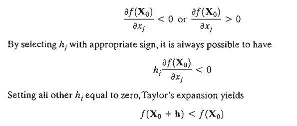
This result contradicts the assumption that X _o is a minimum point. Thus, Ñf(X _o) must equal zero. A similar proof can be established for the maximization case.

Because the necessary condition is also satisfied for inflection and saddle points, it is more appropriate to refer to the points obtained from the solution of Ñf(X_o) = 0 as stationary points. The next theorem establishes the sufficiency conditions for X _o to be an extreme point.

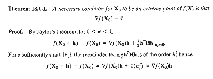
Theorem 18.1-2. A sufficient condition for a stationary point X _o to be an extremum is that the Hessian matrix H evaluated at X _o satisfy the following conditions:

                   i.            H is positive definite if X_ois a minimum point.

                 ii.            H is negative definite I fX_o is a maximum point.

Proof. By Taylor's theorem, for 0 < q < 1,

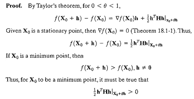
Given that the second partial derivative is continuous, the expression  ½  h^THh must have the same sign at both X_o and X_o + qh. Because h^THhl _Xo defines a quadratic form (see Section 0.3 on the CD), this expression (and hence h^TXh|_Xo+qh) is positive if and only if, H|_x0 is positive-definite. This means that a sufficient condition for the stationary point X _o to be a minimum is that the Hessian matrix, H, evaluated at the same point is positive-definite. A similar proof for the maximization case shows that the corresponding Hessian matrix must be negative-definite.

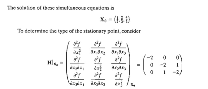
The principal minor determinants of H|_xo have the values -2,4, and -6, respectively. Thus, as shown in Section D.3, HI_Xu is negative-definite and X_o = (1/2, 2/3, 4/3) represents a maximum point.

In general, if H|_x0 is indefinite, X_o must be a saddle point. For nonconclusive cases, X_o mayor may not be an extremum and the sufficiency condition becomes rather involved, because higher-order terms in Taylor's expansion must be considered.

The sufficiency condition established by Theorem 18.1-2 applies to single-variable functions as follows. Given that y_o is a stationary point, then

                               i.            yo is a maximum if f” (yo)  < 0.

                             ii.            yo is a minimum if f" (yo)  > 0.

If f” (y₀) = 0, higher-order derivatives must be investigated as the following theorem requires.

Theorem 18.1-3. Given y_o, a stationary point of f(y), if the first (n  - 1) derivatives are zero and f⁽ⁿ⁾(y_o) != 0, then

                   i.            If n is odd, y_o is an inflection point.

                 ii.            If n is even then y_o is a minimum if f⁽ⁿ⁾(y_o)  > 0 and a maximum if f⁽ⁿ⁾(y_o)  < 0.

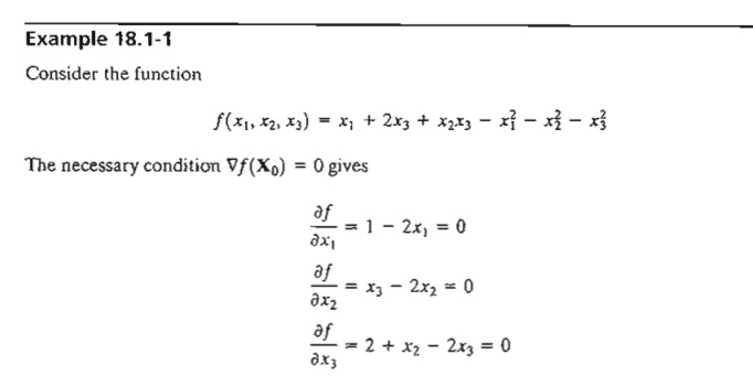
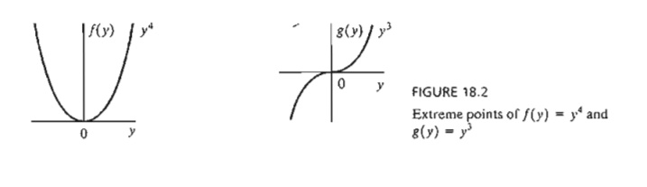
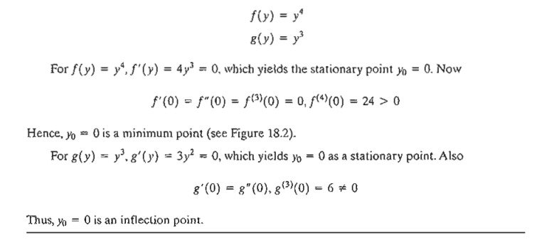
Example 18.1-2

Figure 18.2 graphs the following two functions:

3. Verify that the function

has the stationary points (0, 3, 1), (0, 1, -1), (1,2,0), (2, 1, 1), and (2, 3, -1). Use the sufficiency condition to identify the extreme points.

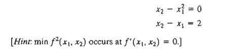
*4. Solve the following simultaneous equations by converting the system to a nonlinear objective function with no constraints.

5. Prove Theorem 18.1-3.

2. The Newton-Raphson Method

In general, the necessary condition equations, Ñ f(X) = 0, may be difficult to solve numerically. The Newton-Raphson method is an iterative procedure for solving simultaneous nonlinear equations.

Consider the simultaneous equations

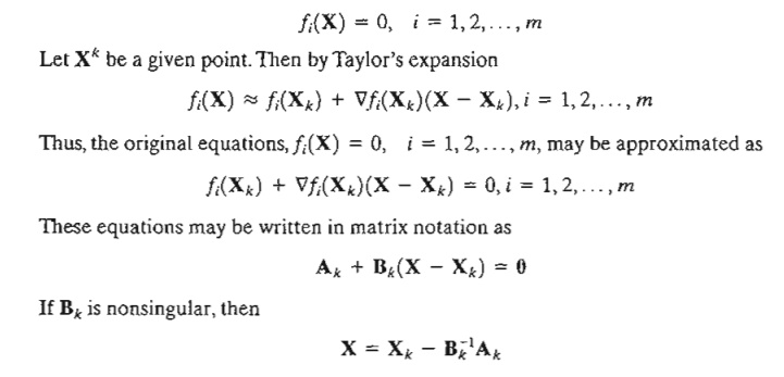
The idea of the method is to start from an initial point X _o and then use the equation above to determine a new point. The process continues until two successive points, X _k and X _{k +1} are approximately equal.

A geometric interpretation of the method is illustrated by a single-variable function in Figure 18.3. The relationship between x_k and x_k+1 for a single-variable function f(x) reduces to

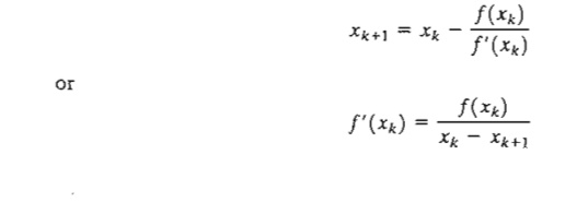
FIGURE 18.3

Illustration of the iterative process in the Newton-Raphson method

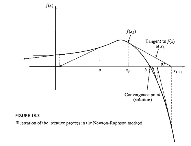
The figure shows that x_k+1 is determined from the slope of f(x) at x_k where tan q = f' (x_k).

One difficulty with the method is that convergence is not always guaranteed unless the function f is well behaved. In Figure 18.3, if the initial point is a, the method will diverge. In general, trial and error is used to locate a "good" initial point.

Example 18.1-3

To demonstrate the use of the Newton-Raphson method, consider determining the stationary points of the function

To determine the stationary points, we need to solve

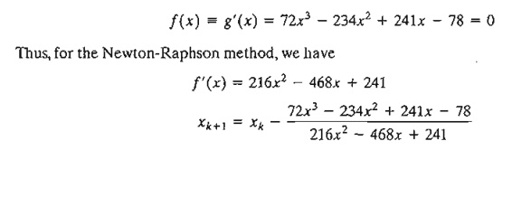
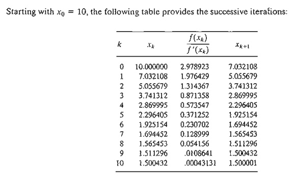
The method converges to x = 1.5. Actually, f(x) has three stationary points at x = 2/3, x = 13/12, and x = 3/2. The remaining two points can be found by selecting different values for initial x_o. In fact, x_o = .5 and x_o = 1 should yield the missing stationary points.

Excel Moment

Template excelNR.xls can be used to solve any single-variable equation. It requires entering f(x)/f' (x) in cell C3. For Example 18.1-3, we enter

The variable x is replaced with A3. The template allows setting a tolerance limit Δ, which specifies the allowable difference between x_k and x_k+1 that signals the termination of the iterations. You are encouraged to use different initial x_o to get a feel of how the method works.

In general, the Newton-Raphson method requires making several attempts before "all" the solutions can be found. In Example 18.1-3, we know beforehand that the equa-tion has three roots. This will not be the case with complex or multi-variable functions, however.

PROBLEM SET 18.1B

1.     Use NewtonRaphson.xls to solve Problem I(c), Set I8.la.

2.     Solve Problem 2(b), Set I8.la by the Newton-Raphson method.