Turing Machines

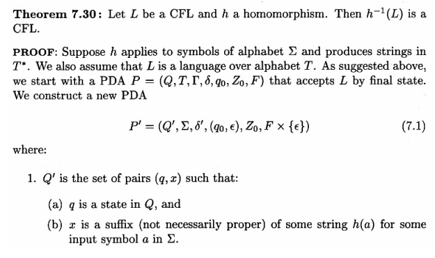
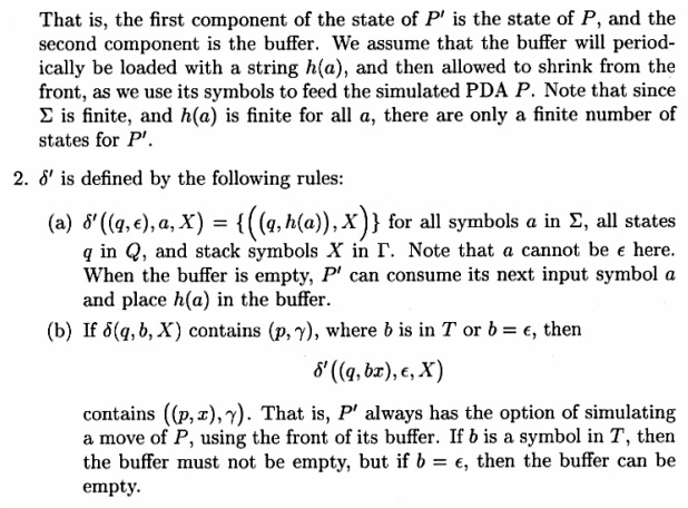
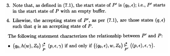
TURING MACHINES

Empty Production Removal 

The productions of context-free grammars can be coerced into a variety of forms without affecting the expressive power of the grammars. If the empty string does not belong to a language, then there is a way to eliminate the productions of the form A → λ from the grammar. If the empty string belongs to a language, then we can eliminate λ from all productions save for the single production S → λ. In this case we can also eliminate any occurrences of S from the right-hand side of productions.

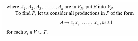
Procedure to find CFG with out empty Productions

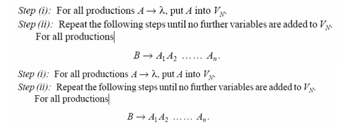
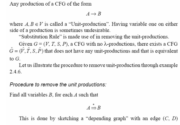
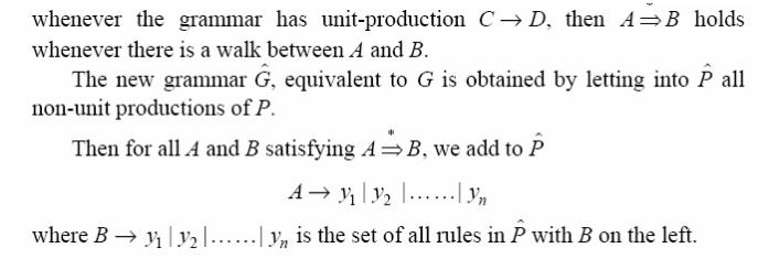
Unit production removal

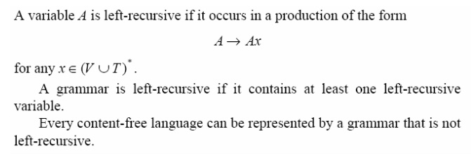
Left Recursion Removal

NORMAL FORMS

Two kinds of normal forms viz., Chomsky Normal Form and Greibach Normal Form (GNF) are

Chomsky Normal Form (CNF)

Any context-free language L without any λ- production is generated by a grammar is which productions are of the form A → BC or A→ a, where A, B ∈VN , and a ∈ V

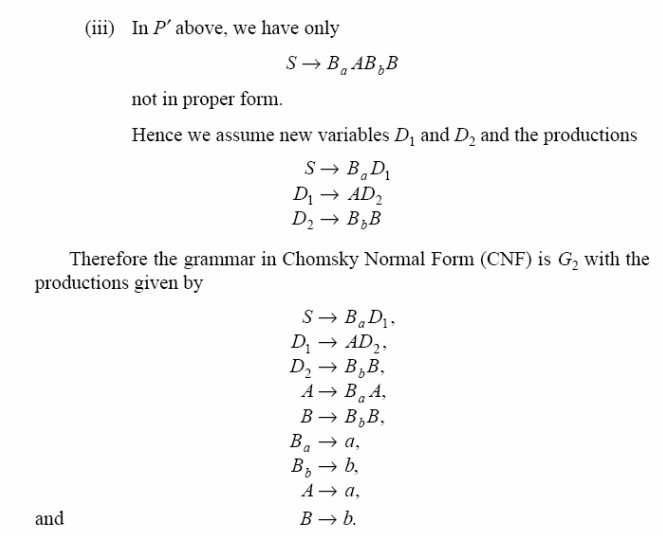
Τ. Procedure to find Equivalent Grammar in CNF

(i)      Eliminate the unit productions, and λ-productions if any,

(ii)     Eliminate the terminals on the right hand side of length two or more.

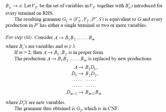
(iii)    Restrict the number of variables on the right hand side of productions to two. Proof:

For Step (i): Apply the following theorem: “Every context free language can be generated by a grammar with no useless symbols and no unit productions”.

At the end of this step the RHS of any production has a single terminal or two or more symbols. Let us assume the equivalent resulting grammar as G = (V_N ,V_T ,P ,S ).

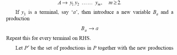
For Step (ii): Consider any production of the form

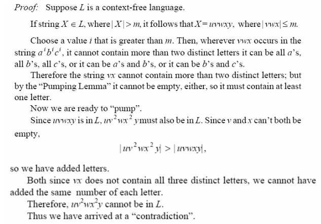
Pumping Lemma for CFG

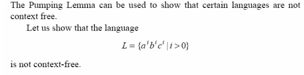
A “Pumping Lemma” is a theorem used to show that, if certain strings belong to a language, then certain other strings must also belong to the language. Let us discuss a Pumping Lemma for CFL. We will show that , if L is a context-free language, then strings of L that are at least ‘m’ symbols long can be “pumped” to produce additional strings in L. The value of ‘m’ depends on the particular language. Let L be an infinite context-free language. Then there is some positive integer ‘m’ such that, if S is a string of L of Length at least ‘m’, then

(i)      S = uvwxy (for some u, v, w, x, y)

(ii)     | vwx| ≤ m

(iii)    | vx| ≥ 1

(iv)    uv iwx i y∈L.

for all non-negative values of i.

It should be understood that

(i)      If S is sufficiently long string, then there are two substrings, v and x, somewhere in S. There is stuff (u) before v, stuff (w) between v and x, and stuff (y), after x.

(ii)     The stuff between v and x won’t be too long, because | vwx | can’t be larger than m.

(iii)    Substrings v and x won’t both be empty, though either one could be.

(iv)    If we duplicate substring v, some number (i) of times, and duplicate x the same number of times, the resultant string will also be in L.

Definitions

A variable is useful if it occurs in the derivation of some string. This requires that

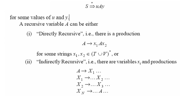
(a) the variable occurs in some sentential form (you can get to the variable if you start from S), and (b) a string of terminals can be derived from the sentential form (the variable is not a “dead end”). A variable is “recursive” if it can generate a string containing itself. For example, variable A is recursive if

Proof of Pumping Lemma

(a) Suppose we have a CFL given by L. Then there is some context-free Grammar G that generates

L. Suppose

(i)      L is infinite, hence there is no proper upper bound on the length of strings belonging to L.

(ii)     L does not contain l.

There are only a finite number of variables in a grammar and the productions for each variable have finite lengths. The only way that a grammar can generate arbitrarily long strings is if one or more variables is both useful and recursive. Suppose no variable is recursive. Since the start symbol is non recursive, it must be defined only in terms of terminals and other variables. Then since those variables are non recursive, they have to be defined in terms of terminals and still other variables and so on.

After a while we run out of “other variables” while the generated string is still finite. Therefore there is an upper bond on the length of the string which can be generated from the start symbol. This contradicts our statement that the language is finite.

Hence, our assumption that no variable is recursive must be incorrect.

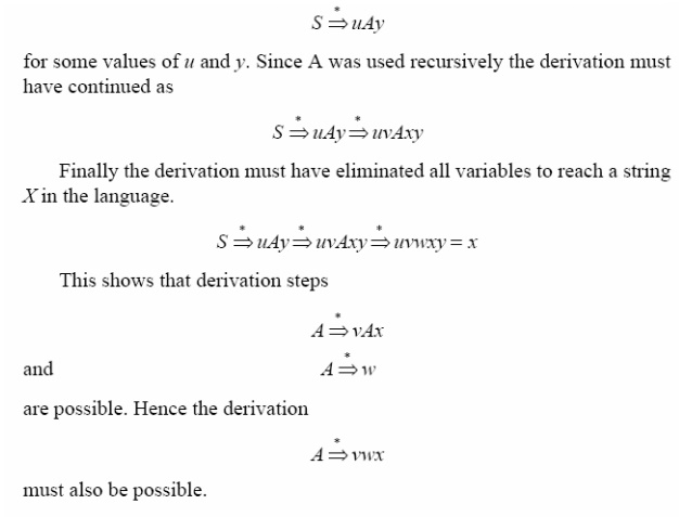
(b) Let us consider a string X belonging to L. If X is sufficiently long, then the derivation of X must have involved recursive use of some variable A. Since A was used in the derivation, the derivation should have started as

Usage of Pumping Lemma

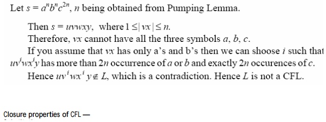
Hence our original assumption, that L is context free should be false. Hence the language L is not context-free.

Example

Check whether the language given by L = {a _mb_mcn : m ≤ n ≤ 2m} is a CFL or not.

Solution

Turing machine:

Informal Definition:

We consider here a basic model of TM which is deterministic and have one-tape. There are many variations, all

The basic model of TM has a finite set of states, a semi-infinite tape that has a leftmost cell but is infinite to the right and a tape head that can move left and right over the tape, reading and writing symbols.

For any input w with |w|=n, initially it is written on the n leftmost (continguous) tape cells. The infinitely many cells to the right of the input all contain a blank symbol, B whcih is a special tape symbol that is not an input symbol. The machine starts in its start state with its head scanning the leftmost symbol of the input w.

Depending upon the symbol scanned by the tape head and the current state the machine makes a move which consists of the following:

•        writes a new symbol on that tape cell,

•        moves its head one cell either to the left or to the right and

•        (possibly) enters a new state.

The action it takes in each step is determined by a transition functions. The machine continues computing (i.e.

•        it decides to "accept" its input by entering a special state called accept or final state or On some inputs the TM many keep on computing forever without ever accepting or rejecting the input, in which case it is said to "loop" on that input

Formal Definition :

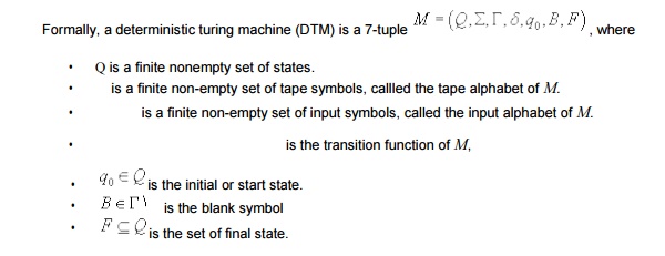
So, given the current state and tape symbol being read, the transition function describes the next state, symbol to be written on the tape, and the direction in which to move the tape head.

Transition function :

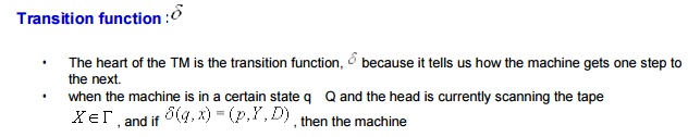
1.      replaces the symbol X by Y on the tape

2.      goes to state p, and

3.      the tape head moves one cell ( i.e. one tape symbol ) to the left ( or right ) if D is L ( or R ).

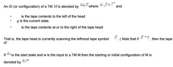
The ID (instantaneous description) of a TM capture what is going out at any moment i.e. it contains all the information to exactly capture the "current state of the computations".

It contains the following:

•        The current state, q

•        The position of the tape head,

•        The constants of the tape up to the rightmost nonblank symbol or the symbol to the left of the head, whichever is rightmost.

Note that, although there is no limit on how far right the head may move and write nonblank symbols on the tape, at any finite time, the TM has visited only a finite prefix of the infinite

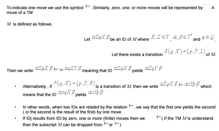
Moves of Turing Machines

Special Boundary Cases

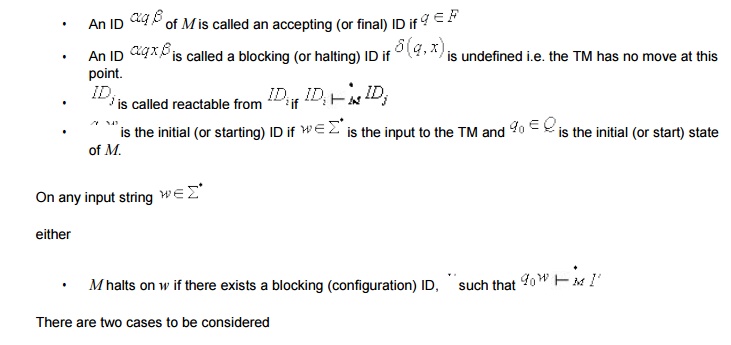
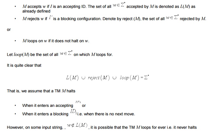
• The representation of IDk contains an accepting state.

The set of strings that M accepts is the language of M, denoted L(M), as defined

More about configuration and acceptance

The Halting Problem

The input to a Turing machine is a string. Turing machines themselves can be written as strings. Since these strings can be used as input to other Turing machines. A “Universal Turing machine” is one whose input consists of a description M of some arbitrary Turing machine, and some input w to which machine M is to be applied, we write this combined input as M + w. This produces the same output that would be produced by M. This is written as

Universal Turing Machine (M + w) = M (w).

As a Turing machine can be represented as a string, it is fully possible to supply a Turing

machine as input to itself, for example M (M). This is not even a particularly bizarre thing to do for example, suppose you have written a C pretty printer in C, then used the Pretty printer on itself. Another common usage is Bootstrapping—where some convenient languages used to write a minimal compiler for some new language L, then used this minimal compiler for L to write a new, improved compiler for language L. Each time a new feature is added to language L, you can recompile and use this new feature in the next version of the compiler. Turing machines sometimes halt, and sometimes they enter an infinite loop.

A Turing machine might halt for one input string, but go into an infinite loop when given some other string. The halting problem asks: “It is possible to tell, in general, whether a given

machine will halt for some given input?” If it is possible, then there is an effective procedure to look at a Turing machine and its input and determine whether the machine will halt with that input. If there is an effective procedure, then we can build a Turing machine to implement it. Suppose we have a Turing machine “WillHalt” which, given an input string M + w, will halt and accept the string if Turing machine M halts on input w and will halt and reject the string if Turing machine M does not halt on input w. When viewed as a Boolean function, “WillHalt (M, w)” halts and returns “TRUE” in the first case, and (halts and) returns “FALSE” in the second.

Theorem

Turing Machine “WillHalt (M, w)” does not exist.

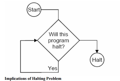
Proof: This theorem is proved by contradiction. Suppose we could build a machine “WillHalt”. Then we can certainly build a second machine, “LoopIfHalts”, that will go into an infinite loop if and only if “WillHalt” accepts its input:

Function LoopIfHalts (M, w):

if WillHalt (M, w) then while true do { }

else

return false;

We will also define a machine “LoopIfHaltOnItSelf” that, for any given input M, representing a Turing machine, will determine what will happen if M is applied to itself, and loops if M will halt in this case.

Function LoopIfHaltsOnItself (M): return LoopIfHalts (M, M):

Finally, we ask what happens if we try:

Func tion Impos sible:

return LoopIfHaltsOnItself (LoopIfHaltsOnItself):

This machine, when applied to itself, goes into an infinite loop if and only if it halts when applied to itself. This is impossible. Hence the theorem is proved.

Programming

The Theorem of “Halting Problem” does not say that we can never determine whether or not a given program halts on a given input. Most of the times, for practical reasons, we could eliminate infinite loops from programs. Sometimes a “meta-program” is used to check another program for potential infinite loops, and get this meta-program to work most of the time.

The theorem says that we cannot ever write such a meta -program and have it work all of the time. This result is also used to demonstrate that certain other programs are also impossible. The basic outline is as follows:

(i) If we could solve a problem X, we could solve the Halting problem

(ii) We cannot solve the Halting Problem

A Turing machine can be "programmed," in much the same manner as a computer is

programmed. When one specifies the function which we usually call δ for a Tm, he is really writing a program for the Tm.

1. Storage in finite Control

The finite control can be used to hold a finite amount of information. To do so, the state is written as a pair of elements, one exercising control and the other storing a symbol. It should be emphasized that this arrangement is for conceptual purposes only. No modification in the definition

of the Turing machine has been made.

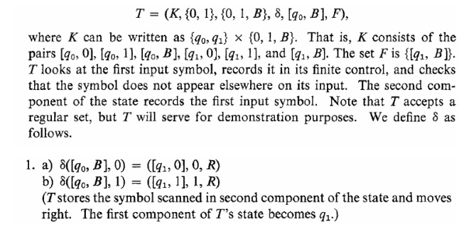
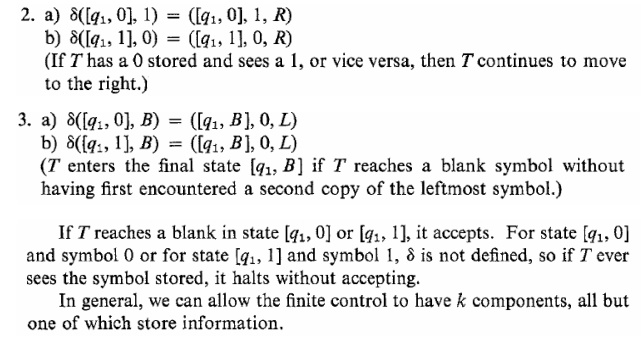
Example

Consider the Turing machine

2. Multiple Tracks

We can imagine that the tape of the Turing machine is divided into k tracks, for any finite k. This arrangement is shown in Fig., with k = 3. What is actually done is that the symbols on the tape are considered as k-tuples. One component for each track.

Example

The tape in Fig. can be imagined to be that of a Turing machine which takes a binary input

greater than 2, written on the first track, and determines if it is a prime. The input is surrounded by ¢ and $ on the first track.

Thus, the allowable input symbols are [¢, B, B], [0, B, B ], [1, B, B ], and [$, B, B]. These

symbols can be identified with ¢, 0, 1, and $, respectively, when viewed as input symbols. The symbol can be represented by [B, B, B ]

To test if its input is a prime, the Tm first writes the number two in binary on the second track and copies the first track onto the third track. Then, the second track is subtracted, as many times as possible, from the third track, effectively dividing the third track by the second and leaving the remainder. If the remainder is zero, the number on the first track is not a prime. If the remainder is nonzero, increase the number on the second track by one.

If now the second track equals the first, the number on the first track is a prime, because it cannot be divided by any number between one and itself. If the second is less than the first, the whole operation is repeated for the new number on the second track. In Fig., the Tm is testing to determine if 47 is a prime. The Tm is dividing by 5; already 5 has been subtracted twice, so 37 appears on the third track.

3. Subroutines