The Assignment Model and The Hungarian Method

THE ASSIGNMENT MODEL

"The best person for the job" is an apt description of the assignment model. The situation can be illustrated by the assignment of workers with varying degrees of skill to jobs. A job that happens to match a worker's skill costs less than one in which the operator is not as skillful. The objective of the model is to determine the minimum-cost assignment of workers to jobs. .

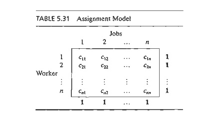
The general assignment model with n workers and n jobs is represented in Table 5.31.

The element c_ij represents the cost of assigning worker i to job j (i, j = 1, 2, ... , n). There is no loss of generality in assuming that the number of workers always

equals the number of jobs, because we can always add fictitious workers or fictitious jobs to satisfy this assumption.

The assignment model is actually a special case of the transportation model in which the workers represent the sources, and the jobs represent the destinations. The supply (demand) amount at each source (destination) exactly equals 1. The cost of "transporting" worker i to job j is c_ij. In effect, the assignment model can be solved directly as a regular transportation model. Nevertheless, the fact that all the supply and demand amounts equal 1 has led to the development of a simple solution algorithm called the Hungarian method. Although the new solution method appears totally un-related to the transportation model, the algorithm is actually rooted in the simplex method, just as the transportation model is.

1. The Hungarian Method

We will use two examples to present the mechanics of the new algorithm. The next section provides a simplex-based explanation of the procedure.

Example 5.4-1

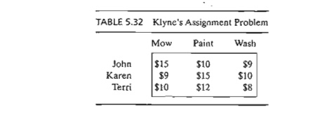
Joe Klyne's three children, John, Karen, and Terri, want to earn some money to take care of personal expenses during a school trip to the local zoo. Mr. Klyne has chosen three chores for his children: mowing the lawn, painting the garage door, and washing the family cars. To avoid antic-ipated sibling competition, he asks them to submit (secret) bids for what they feel is fair pay for each of the three chores. The understanding is that aU three children will abide by their father's decision as to who gets which chore. Table 5.32 summarizes the bids received. Based on this information, how should Mr. Klyne assign the chores?

The assignment problem will be solved by the Hungarian method.

Step 1. For the original cost matrix, identify each row's minimum, and subtract it from all the entries of the row. .

Step 2. For the matrix resulting from step 1, identify each column's minimum, and subtract it from all the entries of the column.

Step 3. Identify the optimal solution as the feasible assignment associated with the zero ele-ments of the matrix obtained in step 2.

Let p_i and q_j be the minimum costs associated with row i and column j as defined in steps 1 and 2, respectively. The row minimums of step 1 are computed from the original cost matrix as shown in Table 5.33.

Next, subtract the row minimum from each respective row to obtain the reduced matrix in Table 5.34.

The application of step 2 yields the column minimums in Table 5.34. Subtracting these values from the respective columns, we get the reduced matrix in Table 5.35.

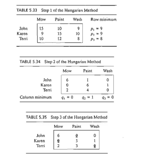
The cells with underscored zero entries provide the optimum solution. This means that John gets to paint the garage door, Karen gets to mow the lawn, and Terri gets to wash the family cars. The total cost to Mr. Klyne is 9 + 10 + 8 = $27. This amount also will always equal (p₁ + p₂ + p₃) + (q₁ + q₂ + q₃) = (9 + 9 + 8)+(0 + 1 + 0) = $27. (A justification of this result is given in the next section.)

The given steps of the Hungarian method work well in the preceding example because the zero entries in the final matrix happen to produce a feasible assignment (in the sense that each child is assigned a distinct chore). In some cases, the zeros created by steps 1 and 2 may not yield a feasible solution directly, and further steps are needed to find the optimal (feasible) assignment. The following example demonstrates this situation.

Example 5.4-2

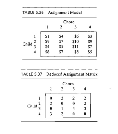
Suppose that the situation discussed in Example 5.4-1 is extended to four children and four chores. Table 5.36 summarizes the cost elements of the problem.

The application of steps 1 and 2 to the matrix in Table 5.36 (using p₁ = 1, p₂ = 7, p₃ = 4, p₄ = 5, q₁ = 0, q₂ = 0, q₃ = 3, and q₄ = 0) yields the reduced matrix in Table 5.37 (verify!).

The locations of the zero entries do not allow assigning unique chores to all the children. For example, if we assign child 1 to chore 1, then column 1 will be eliminated, and child 3 will not have a zero entry in the remaining three columns. This obstacle can be accounted for by adding the following step to the procedure outlined in Example 5.4-1:

Step 2a. If no feasible assignment (with all zero entries) can be secured from steps 1 and 2,

(i) Draw the minimum number of horizontal and vertical lines in the last reduced matrix that will cover all the zero entries.

(ii) Select the smallest uncovered entry, subtract it from every uncovered entry, then add it to every entry at the intersection of two lines.

(iii) If no feasible assignment can be found among the resulting zero entries, repeat step 2a. Otherwise, go to step 3 to determine the optimal assignment.

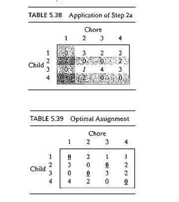
The application of step 2a to the last matrix produces the shaded cells in Table 5.38. The smallest unshaded entry (shown in italics) equals 1. 111is entry is added to the bold intersection cells and subtracted from the remaining shaded cells to produce the matrix in Table 5.39.

The optimum solution (shown by the underscored zeros) calls for assigning child 1 to chore 1, child 2 to chore 3, child 3 to chore 2, and child 4 to chore 4. The associated optimal cost is 1 + 10 + 5 + 5 = $21. The same cost is also determined by summing the p_is, the q_is, and the entry that was subtracted after the shaded cells were determined-that is, (1 + 7 + 4 + 5) + (0 + 0 + 3 + 0) + (1) = $21.

AMPL Moment.

File amplEx5.4-2.txt provides the AMPL model for the assignment model. The model is very similar to that of the transportation model.

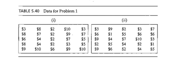
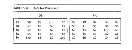
PROBLEM SET 5.4A

1. Solve the assignment models in Table 5.40.

a. Solve by the Hungarian method.

b. TORA Experiment. Express the problem as an LP and solve it with TORA.

c. TORA Experiment. Use TORA to solve the problem as a transportation model.

d. Solver Experiment. Modify Excel file solverEx5.3-l.xls to solve the problem.

e. AMPL Experiment. Modify ampIEx5.3-1b.txt to solve the problem.

2. JoShop needs to assign 4 jobs to 4 workers. The cost of performing a job is a function of the skills of the workers. Table 5.41 summarizes the cost of the assignments. Worker 1 cannot do job 3 and worker 3 cannot do job 4. Determine the optimal assignment using the Hungarian method.

3. In the JoShop model of Problem 2, suppose that an additional (fifth) worker becomes available for performing the four jobs at the respective costs of $60, $45, $30, and $80. Is it economical to replace one of the current four workers with the new one?

4.In the model of Problem 2, suppose that JoShop has just received a fifth job and that the respective costs of performing it by the four current workers are $20, $10, $20, and $80. Should the new job take priority over any of the four jobs JoShop already has?

*5. A business executive must make the four round trips listed in Table 5.42 between the head office in Dallas and a branch office in Atlanta.

The price of a round-trip ticket from Dallas is $400. A discount of 25% is granted if the dates of arrival and departure of a ticket span a weekend (Saturday and Sunday). If the stay in Atlanta lasts more than 21 days, the discount is increased to 30%. A one-way

ticket between Dallas and Atlanta (either direction) costs $250. How should the execu-tive purchase the tickets?

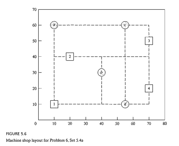
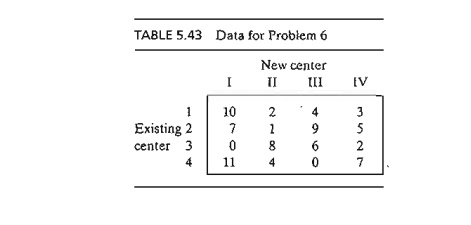
*6. Figure 5.6 gives a schematic layout of a machine shop with its existing work centers des-ignated by squares 1,2,3, and 4. Four new work centers, I, II, III, and IV, are to be added to the shop at the locations designated by circles a, b, c, and d. The objective is to assign the new centers to the proposed locations to minimize the total materials handling traf-fic between the existing centers and the proposed ones. Table 5.43 summarizes the frequency of trips between the new centers and the old ones. Materials handling equip-ment travels along the rectangular aisles intersecting at the locations of the centers. For example, the one-way travel distance (in meters) between center 1 and location b is 30 + 20 = 50 m.

7. In the Industrial Engineering Department at the University of Arkansas, INEG 4904 is a capstone design course intended to allow teams of students to apply the knowledge and skills learned .in the undergraduate curriculum to a practical problem. The members of each team select a project manager, identify an appropriate scope for their project, write and present a proposal, perform necessary tasks for meeting the project objectives, and write and present a final report. The course instructor identifies potential projects and provides appropriate information sheets for each, including contact at the sponsoring or-ganization, project summary, and potential skills needed to complete the project. Each design team is required to submit a report justifying the selection of team members and the team manager. The report also provides a ranking for each project in order of prefer-ence, including justification regarding proper matching of the team's skills with the pro-ject objectives. In a specific semester, the following projects were identified: Boeing F-lS, Boeing F-18, Boeing Simulation, Cargil, Cobb-Vantress, ConAgra, Cooper, DaySpring (layout), DaySpring (material handling), IB. Hunt, Raytheon, Tyson South, Tyson East, Wal-Mart, and Yellow Transportation. The projects for Boeing and Raytheon require U.S. citizenship of all team members. Of the eleven design teams available for this semester, four do not meet this requirement.

Devise a procedure for assigning projects to teams and justify the arguments you use to reach a decision.

2. Simplex Explanation of the Hungarian Method

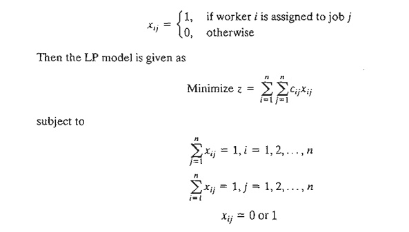
The assignment problem in which n workers are assigned to n jobs can be represented as an LP model in the following manner: Let c_ij be the cost of assigning worker i to job j, and define

The optimal solution of the preceding LP model remains unchanged if a constant is added to or subtracted from any row or column of the cost matrix (c_ij). To prove this point, let p_i and q_j be constants subtracted from row i and column j. Thus, the cost element c_ij is changed to

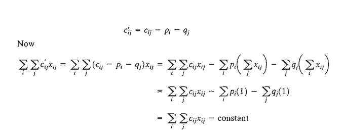
Because the new objective function differs from the original one by a constant, the optimum values of x_ij must be the same in both cases. The development thus shows that steps 1 and 2 of the Hungarian method, which call for subtracting p_i from row i and then subtracting q_j from column j, produce an equivalent assignment model. In this regard, if a feasible solution can be found among the zero entries of the cost matrix created by steps 1 and 2, then it must be optimum because the cost in the modified matrix cannot be less than zero.

If the created zero entries cannot yield a feasible solution (as Example 5.4-2 demonstrates), then step 2a (dealing with the covering of the zero entries) must be ap-plied. The validity of this procedure is again rooted in the simplex method of linear programming and can be explained by duality theory (Chapter 4) and the complementary slackness theorem (Chapter 7). We will not present the details of the proof here because they are somewhat involved.

The reason (p₁ + p₂ + ... + p_n) + (q₁ + q₂ + ... + q_n) gives the optimal objective value is that it represents the dual objective function of the assignment model. This result can be seen through comparison with the dual objective function of the transportation model given in Section 5.3.4. [See Bazaraa and Associates (1990, pp. 499-508) for the details.]