Chapter: Database Management Systems : SQL & Query Optimization
Query Processing and Optimization (QPO)
Query Processing and Optimization (QPO)
Basic
idea of QPO
In
SQL, queries are expressed in high level declarative form
QPO translates a SQL
query to an execution plan
•
over physical data model
•
using operations on file-structures, indices, etc.
Ideal
execution plan answers Q in as little time as possible
A ROLLBACK does exactly the opposite of
COMMIT. It ends the transaction but undoes any changes made during the
transaction. All transaction locks acquired on tables are released.
Constraints:
QPO overheads are small
•
Computation time for QPO steps << that for execution plan
Three Key Concepts in QPO
Building blocks
Most cars have few motions, e.g.
forward, reverse
Similar most DBMS have few building
blocks:
• select (point query, range
query), join, sorting, ...
A SQL queries is decomposed in building blocks 2. Query processing
strategies for building blocks
Cars have a few gears for forward
motion: 1st, 2nd, 3rd, overdrive
DBMS keeps a few processing
strategies for each building block
• e.g. a point query can be answer
via an index or via scanning data-file 3. Query optimization
Automatic transmission tries to
picks best gear given motion parameters
For each building block of a given
query, DBMS QPO tries to choose
• ―Most efficient‖
strategy given data
• Parameter examples:
Table size, avai
Ex. Index search is chosen for a
point query if the index is available
QPO Challenges
Choice of building blocks
SQL Queries are based on relational
algebra (RA)
Building blocks of RA are select,
project, join
• Details in section 3.2 (Note
symbols sigma, pi and join) SQL3 adds new building blocks like transitive
closure
• Will be discussed in chapter 6
Choice of processing strategies for
building blocks
Too many strategies=> higher
complexity
Commercial DBMS have a total of 10
to 30 strategies
• 2 to 4 strategies for each
building block
How to choose
the ―best‖icable
ones?strategy from amo
May use a fixed priority scheme
May use a simple cost model based
on DBMS parameters
QPO Challenges in SDBMS
Building Blocks for spatial queries
Rich set of spatial data types,
operations
A consensus on
―building blocks‖ is
lac
Current choices include spatial select, spatial join, nearest neighbor
Choice of strategies
Limited choice for some building blocks, e.g. nearest neighbor Choosing
best strategies
Cost models are more complex since
• Spatial
Queries are both CPU and I/O intensive
• while
traditional queries are I/O intensive
Cost models of spatial strategies
are in not mature.
Query Processing and Optimizer process
•
A site-seeing trip
•
Start : A SQL Query
•
End: An execution plan
•
Intermediate Stopovers
•
query trees
•
logical tree transforms
•
strategy selection
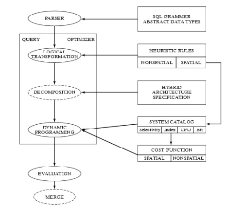
Query Trees
•
Nodes = building blocks of (spatial)
queries
•
symbols sigma, pi and join
•
Children = inputs to a building block
•
Leafs = Tables
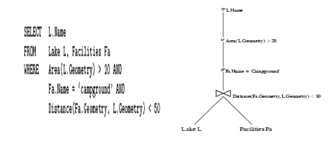
Example SQL query and its query tree follows:
Logical Transformation of Query Trees
•
Motivation
•
Transformation do not change the answer
of the query
•
But can reduce computational cost by
•
reducing data produced by sub-queries
•
reducing computation needs of parent
node
•
Example Transformation
•
Push down select operation below join
•
Example: Fig. 5.4 (compare w/ Fig 5.3,
last slide)
•
Reduces size of table for join operation
•
Other common transformations
•
Push project down
•
Reorder join operations
•
Traditional logical transform rules
•
For relational queries with simple data
types and operations
•
CPU costs are much smaller and I/O costs
•
Need to be reviewed for spatial queries
•
complex data types, operations
•
CPU cost is higher
•
Execution Plans
An execution plan has 3 components
A query tree
A strategy selected for each non-leaf node
An ordering of evaluation of non-leaf nodes
Query Decomposition
Normalization
o
manipulate query quantifiers and qualification
Analysis
o detect and reject ―incorrect‖ queries o possible
for only a subset of relational calculus
Simplification
o eliminate redundant predicates
Restructuring
o
calculus query Þ algebraic query
o more than one translation is possible o use
transformation rules
Trends in Query Processing and
Optimization
Motivation
SDBMS
and GIS are invaluable to many organizations
Price
of success is to get new requests from customers
•
to support new computing hardware and
environment
•
to support new applications
New
computing environments
Distributed
computing
Internet
and web
Parallel
computers
New
applications
Location
based services, transportation
Data
Mining
Raster
data
Distributed Spatial Databases
Distributed
Environments
Collection
of autonomous heterogeneous computers
Connected
by networks
Client-server
architectures
•
Server computer provides well-defined
services
•
Client computers use the services
New
issues for SDBMS
Conceptual
data model -
• Translation between heterogeneous
schemas Logical data model
•
Naming and querying tables in other
SDBMSs
•
Keeping copies of tables (in other
SDBMs) consistent with original table
Query
Processing and Optimization
•
Cost of data transfer over network may
dominate CPU and I/O costs
•
New strategies to control data transfer
costs
n
Process for heuristics optimization
1.
The parser of a high-level query
generates an initial internal representation;
2.
Apply heuristics rules to optimize the
internal representation.
3.
A query execution plan is generated to
execute groups of operations based on the access paths available on the files
involved in the query.
n
The main heuristic is to apply
first the operations that reduce the size of intermediate results.
E.g., Apply SELECT and PROJECT operations before
applying the JOIN or other binary operations.
n
Query tree:
n
A tree data structure that
corresponds to a relational algebra expression. It represents the input
relations of the query as leaf nodes of the tree, and represents
the relational
algebra operations as internal nodes.
n
An execution of the query tree
consists of executing an internal node operation whenever its operands are
available and then replacing that internal node by the relation that results
from
executing the operation.
Query graph
A graph data structure that corresponds to a
relational calculus expression. It does not indicate an order on which
operations to perform first. There is only a single graph corresponding
to each query.
n
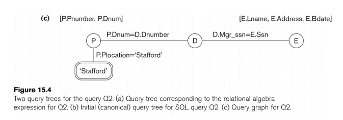
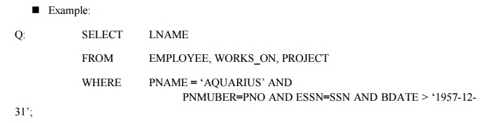
Example:
n
For every project located in “Stafford
department number and the department ma
n
Relation algebra:
pPNUMBER, DNUM, LNAME, ADDRESS, BDATE (((sPLOCATION=“STAFFORD‘(PROJECT))
DNUM=DNUMBER
(DEPARTMENT)) MGRSSN=SSN
(EMPLOYEE))
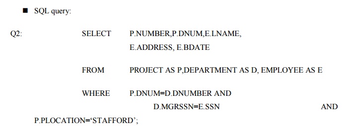
P.PLOCATION=“STAFFORD‘;
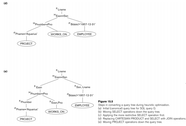
Heuristic Optimization of Query Trees:
n
The same query could correspond to
many different relational algebra expressions — and hence many different query
trees.
n The task of heuristic optimization of query trees is to find a final query tree that is efficient to execute.
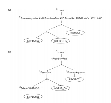
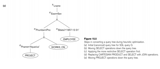
n
General Transformation Rules for
Relational Algebra Operations:
1. Cascade
of s: A conjunctive selection condition can be broken up into a cascade
(sequence) of individual s operations:
n
s c1 AND c2 AND ... AND cn(R)
= sc1 (sc2 (...(scn(R))...) )
2. Commutativity
of s: The s operation is commutative:
n
sc1 (sc2(R))
= sc2 (sc1(R))
3. Cascade
of p: In a cascade (sequence) of p operations, all but the last one can be
ignored:
n
pList1 (pList2
(...(pListn(R))...) ) = pList1(R)
4. Commuting
s with p: If the selection condition c involves only the attributes A1, ..., An
in the projection list, the two operations can be commuted:
pA1,
A2, ..., An (sc (R)) = sc (pA1, A2, ..., An (R))
.
Commutativity of ( and x ): The operation is commutative as is the x
operation:
R C S = S C R; R x S = S x R
6.
Commuting s with (or x ): If all the
attributes in the selection condition c involve only the attributes of one of
the relations being joined—say, R—the two operations can be commuted as follows:
sc ( R S ) = (sc (R)) S
n
Alternatively, if the selection
condition c can be written as (c1 and c2), where condition c1 involves only the
attributes of R and condition c2 involves only the attributes of S, the
operations commute as follows:
n
sc ( R S ) =
(sc1 (R)) (sc2 (S))
n
Commuting p with (or x): Suppose that the projection list is L = {A1, ...,
An, B1, ..., Bm},
where A1, ..., An are
attributes of R and B1, ..., Bm are attributes of S. If the join condition c
involves only attributes in L, the two operations can be commuted as follows:
pL ( R C S ) = (pA1, ..., An (R)) C (p B1, ..., Bm (S))
n
If the join condition C contains
additional attributes not in L, these must be added to the projection list, and
a final p operation is needed.
Commutativity of set operations: The
set operations–‖is notυ
9. Associativity of ,
x, υ, and ∩ : Th if q stands for any one of these four operations (throughout
the expression), we have
( R q S ) q T = R q ( S q T )
10. Commuting s with
set operations:–.IfqstandsThe s for any one of these three operations, we have
sc ( R q S ) = (sc
(R)) q (sc (S))
The p
operation commutes withpL( υR. υ LS(R)) =υ
(pL
(S))
Converting a (s, x) sequence into : If the condition c of a s that follows a x
Corresponds to a join condition, convert the (s, x) sequence into a as follows:
(sC
(R x S)) = (R C S)
Other transformations
Outline of a Heuristic Algebraic Optimization
Algorithm:
1.
Using rule 1, break up any select
operations with conjunctive conditions into a cascade of select operations.
2.
Using rules 2, 4, 6, and 10 concerning
the commutativity of select with other operations, move each select operation
as far down the query tree as is permitted by the attributes involved in the
select condition.
3.
Using rule 9 concerning associativity of
binary operations, rearrange the leaf nodes of the tree so that the leaf node
relations with the most restrictive select operations are executed first in the
query tree representation.
4.
Using Rule 12, combine a Cartesian
product operation with a subsequent select operation in the tree into a join
operation.
5.
Using rules 3, 4, 7, and 11 concerning
the cascading of project and the commuting of project with other operations,
break down and move lists of projection attributes down the tree as far as possible
by creating new project operations as needed.
Identify subtrees that represent groups of
operations that can be executed by a single algorithm.
n
Heuristics for Algebraic
Optimization:
1.
The main heuristic is to apply first the
operations that reduce the size of intermediate results.
2.
Perform select operations as early as
possible to reduce the number of tuples and perform project operations as early
as possible to reduce the number of attributes. (This is done by moving select
and project operations as far down the tree as possible.)
3.
The select and join operations that are
most restrictive should be executed before other similar operations. (This is
done by reordering the leaf nodes of the tree among themselves and adjusting
the rest of the tree appropriately.)
n
Query Execution Plans
1.
An execution plan for a relational
algebra query consists of a combination of the relational algebra query tree
and information about the access methods to be used for each relation as well
as the methods to be used in computing the relational operators stored in the
tree.
2.
Materialized evaluation:
the result of an operation is stored as a temporary relationPipelined
evaluation: as the result of an operator is produced, it is forwarded to
the next operator in sequence.
n
Cost-based query
optimization:
n
Estimate and compare the costs of
executing a query using different execution strategies and choose the strategy
with the lowest cost estimate.
n
(Compare to heuristic query
optimization)
n
Issues
n
Cost function
Number of execution strategies to be considered
n
Cost Components for Query Execution
1.
Access cost to secondary storage
2.
Storage cost
3.
Computation cost
4.
Memory usage cost
5.
Communication cost
n
Note: Different database systems
may focus on different cost components.
n
Catalog Information Used in Cost
Functions
1.
Information about the size of a file
n
number of records (tuples) (r),
n
record size (R),
n
number of blocks (b)
n
blocking factor (bfr)
2.
Information about indexes and indexing
attributes of a file
n
Number of levels (x) of each
multilevel index
n
Number of first-level index blocks
(bI1)
n
Number of distinct values (d) of an
attribute
n
Selectivity (sl) of an attribute
n
Selection cardinality (s) of an
attribute. (s = sl * r)
n
Examples of Cost Functions for
SELECT
n
S1. Linear search (brute force)
approach
1.
CS1a = b;
2.
For an equality condition on a key, CS1a
= (b/2) if the record is found; otherwise CS1a = b.
n
S2. Binary search:
1.
CS2 = log2b +
(s/bfr)–For an equality condition on a unique (key) attribute, CS2
=log2b
n
S3. Using a primary index (S3a) or
hash key (S3b) to retrieve a single record
1.
CS3a = x + 1; CS3b
= 1 for static or linear hashing;
CS3b = 1 for extendible hashing;
n
S4. Using an ordering index to
retrieve multiple records:
n
For the comparison condition on a
key field with an ordering index, CS4 = x + (b/2)
n
S5. Using a clustering index to
retrieve multiple records:
CS5 = x +
┌ (s/bfr) ┐
n
S6. Using a secondary (B+-tree)
index:
n
For an equality comparison, CS6a
= x + s;
n
For an comparison condition such as
>, <, >=, or <=,
n
CS6a = x + (bI1/2)
+ (r/2)
n
S7. Conjunctive selection:
n
Use either S1 or one of the methods
S2 to S6 to solve.
n
For the latter case, use one
condition to retrieve the records and then check in the memory buffer whether
each retrieved record satisfies the remaining conditions in the conjunction.
n
S8. Conjunctive selection using a
composite index:
n
Same as S3a, S5 or S6a, depending
on the type of index.
Examples of
Cost Functions for
Join
selectivity (js)
js = | (R C S) | / | R x S |
= | (R C S) | / (|R| * |S |)
n
If condition C does not exist, js =
1;
n
If no tuples from the relations
satisfy condition C, js = 0;
n
Usually, 0 <= js <= 1;
n
Size of the result file after join
| (R C S) | = js * |R| * |S
|
n
J1. Nested-loop join:
n
CJ1 = bR + (bR*bS)
+ ((js* |R|* |S|)/bfrRS)
n
(Use R for outer loop)
n
J2. Single-loop join (using an
access structure to retrieve the matching record(s))
n
If an index exists for the join
attribute B of S with index levels xB, we can retrieve each record s
in R and then use the index to retrieve all the matching records t from S that
satisfy t[B] = s[A].
n
The cost depends on the type of
index.
n
J2. Single-loop join (contd.)
n
For a secondary index,
n
CJ2a = bR +
(|R| * (xB + sB)) + ((js* |R|* |S|)/bfrRS);
n
For a clustering index,
n
CJ2b = bR + (|R| * (xB + (sB/bfrB)))
+ ((js* |R|* |S|)/bfrRS);
n
For a primary index,
n
CJ2c = bR + (|R| * (xB + 1)) +
((js* |R|* |S|)/bfrRS);
n
If a hash key exists for one of the
two join attributes — B of S
n
CJ2d = bR + (|R| * h) + ((js* |R|*
|S|)/bfrRS);
n
J3. Sort-merge join:
n
CJ3a = CS + bR
+ bS + ((js* |R|* |S|)/bfrRS);
n
(CS: Cost for sorting files)
n
Multiple Relation
Queries and Join Ordering
n
A query joining n relations will
have n-1 join operations, and hence can have a large number of different join
orders when we apply the algebraic transformation rules.
n
Current query optimizers typically
limit the structure of a (join) query tree to that of left-deep (or right-deep)
trees.
n
Left-deep tree:
n
A binary tree where the right child
of each non-leaf node is always a base relation.
n
Amenable to pipelining
Could utilize any access paths on the base relation
(the right child) when executing the join.
n
Oracle DBMS V8
n
Rule-based query
optimization: the optimizer chooses execution plans
based on heuristically ranked operations.
n
(Currently it is being phased out)
n
Cost-based query
optimization: the optimizer examines alternative access
paths and operator algorithms and chooses the execution plan with lowest
estimate cost.
n
The query cost is calculated based
on the estimated usage of resources such as I/O, CPU and memory needed.
n
Application developers could
specify hints to the ORACLE query optimizer.
n
The idea is that an application
developer might know more information about the data.
n
Semantic Query
Optimization:
n
Uses constraints specified on the
database schema in order to modify one query into another query that is more efficient
to execute.
n
Consider the following SQL query,
SELECT E.LNAME, M.LNAME
FROM
EMPLOYEE E M
WHERE E.SUPERSSN=M.SSN AND E.SALARY>M.SALARY
Explanation:
Suppose that we had a constraint on the database schema that stated that no
employee
can
earn more than his or her direct supervisor. If the semantic query optimizer
checks
for
the existence of this constraint, it need not execute the query at all because
it knows that the result of the query will be empty. Techniques known as
theorem proving can be used for this purpose.
Related Topics