Normal Distribution

Distribution

The following are the two types of Theoretical distributions :

1. Discrete distribution  2. Continous distribution

Continuous distribtuion

The binomial and Poisson distributions discussed in the previous chapters are the most useful theoretical distributions for discrete variables. In order to have mathematical distributions suitable for dealing with quantities whose magnitudes vary continuously like weight, heights of individual, a continuous distribution is needed. Normal distribution is one of the most widely used continuous distribution.

Normal distribution is the most important and powerful of all the distribution in statistics. It was first introduced by De Moivre in 1733 in the development of probability. Laplace (1749-1827) and Gauss (1827-1855) were also associated with the development of Normal distribution.

NORMAL DITRIBUTION

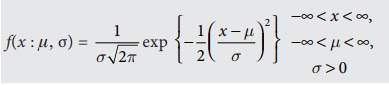
Definition 7.3

A random variable X is said to follow a normal distribution with parameters mean and variance σ² , if its probability density function is given by

Normal distribution is diagrammatically represented as follows :

Normal distribution is a limiting case of Binomial distribution under the following conditions:

(i) n, the number of trials is infinitely large, i.e. n → ∞

(ii) neither p (or q) is very small,

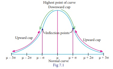
The normal distribution of a variable when represented graphically, takes the shape of a symmetrical curve, known as the Normal Curve. The curve is asymptotic to x-axis on its either side.

Chief Characterisitics or Properties of Normal Probabilty distribution and Normal probability Curve .

The normal probability curve with mean μ and standard deviation σ has the following properties:

(i) the curve is bell- shaped and symmetrical about the line x=u

(ii) Mean, median and mode of the distribution coincide.

(iii) x – axis is an asymptote to the curve. ( tails of the cuve never touches the horizontal (x) axis)

(iv) No portion of the curve lies below the x-axis as f (x) being the probability function can never be negative.

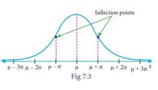
(v) The Points of inflexion of the curve are x = ± µ σ

(vi)  The curve of a normal distribution has a single peak i.e it is a unimodal.

(vii) As x increases numerically, f (x) decreases rapidly, the maximum probability occurring at the point x = μ and is given by [p(x)]max = 1 / σ √2π

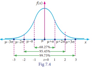
(viii) The total area under the normal curve is equal to unity and the percentage distribution of area under the normal curve is given below

(a) About 68.27% of the area falls between μ – σ and μ + σ

P(μ – σ < X < μ + σ) = 0.6826

(b) About 95.5% of the area falls between μ – 2σ and μ + 2σ

P(μ – 2σ < X < μ + 2σ) = 0.9544

(c) About 99.7% of the area falls between μ – 3σ and μ + 3σ

P(μ – 3σ < X < μ + 3σ) = 0.9973

STANDARD NORMAL DISTRIBUTION

A random variable Z = (X–μ)/σ follows the standard normal distribution. Z is called the standard normal variate with mean 0 and standard deviation 1 i.e Z ~ N(0,1). Its Probability density function is given by :

1. The area under the standard normal curve is equal to 1.

2. 68.26% of the area under the standard normal curve lies between z = –1 and Z =1

95.44% of the area lies between Z = –2 and Z = 2

99.74% of the area lies between Z = –3 and Z = 3

Example 7.21

What is the probability that a standard normal variate Z will be

(i) greater than 1.09

(ii) less than -1.65

(iii) lying between -1.00 and 1.96

(iv) lying between 1.25 and 2.75

Solution :

(i) greater than 1.09

The total area under the curve is equal to 1 , so that the total area to the right Z = 0 is 0.5 (since the curve is symmetrical). The area between Z = 0 and 1.09 (from tables) is 0.3621

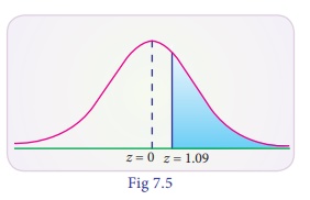
P(Z > 1.09) = 0.5000 - 0.3621 = 0.1379

The shaded area to the right of Z = 1.09 is the probability that Z will be greater than 1.09

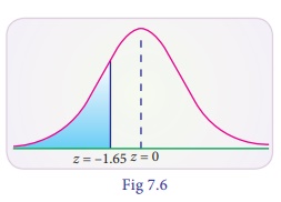
(ii) less than –1.65

The area between -1.65 and 0 is the same as area between 0 and 1.65. In the table the area between zero and 1.65 is 0.4505 (from the table). Since the area to the left of zero is 0.5 , P(Z< 1.65) = 0.5000 – 0.4505 = 0.0495.

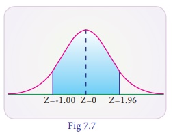
(iii) lying between -1.00 and 1.96

The probability that the random variable Z in between -1.00 and 1.96 is found by adding the corresponding areas :

Area between -1.00 and 1.96 = area between (-1.00 and 0) + area betwn (0 and 1.96)

P(–1.00 < Z < 1.96) = P(–1.00 < Z < 0) + P(0 < Z < 1.96) = 0.3413 + 0.4750 (by tables)

= 0.8163

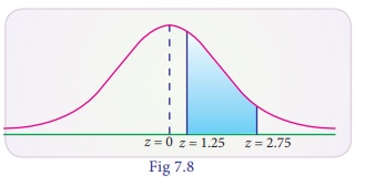
(iv) lying between 1.25 and 2.75

Area between Z = 1.25 and 2.75 = area betwn (z = 0 and z = 2.75) – area betwn (z=0 and z = 1.25)

P(1.25 < Z < 2.75) = P(0 < Z < 2.75) – P(0 < Z < 1.25)

= 0.4970 - 0.3944  = 0.1026

Example 7.22

If X is a normal variate with mean 30 and SD 5. Find the probabilities that (i) 26 ≤ X ≤ 40 (ii) X > 45

Solution :

Here mean μ= 30 and standard deviation σ = 5

(i) When X = 26 Z = ( X − µ ) / σ = (26 – 30)/5 = –0.8

And when X = 40 , Z = [40 – 30] /5 = 2

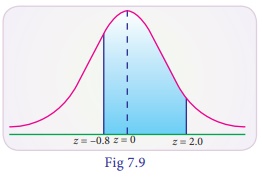
Therefore,

P(26<X<40) ) = P(–0.8 ≤ Z < 2)

= P(–0.8 ≤ Z ≤ 0) + p(0 ≤ Z ≤ 2)

= P(0 ≤ Z ≤ 0.8) + P(0 ≤ Z ≤ 2)

= 0.2881 + 0.4772 (By tables)

= 0.7653

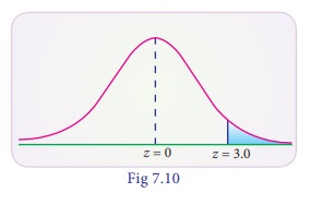
(ii) The probability that X≥45

When X = 45

Z = [X − µ] / σ = [45 – 30] / 5 = 3

=P( X ≥ 45) = P(Z ≥ 3)

= 0.5 – 0.49865

= 0.00135

Example 7.23

The average daily sale of 550 branch offices was Rs.150 thousand and standard deviation is Rs. 15 thousand. Assuming the distribution to be normal, indicate how many branches have sales between

(i)₹ 1,25,000 and ₹ 1, 45, 000

(i) ₹ 1,40,000 and ₹ 1,60,000

Solution :

Given that mean μ= 150 and standard deviation σ= 15

(i) when X = 125 thousand

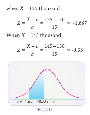
Area between Z = 0 and Z = -1.67 is 0.4525

Area between Z = 0 and Z = -0.33 is 0.1293

P(–1.667 ≤ Z ≤ –0.33) = 0.4525 – 0.1293

= 0.3232

Therefore the number of branches having sales between 125 thousand and 145 thousand is 550 × 0.3232 = 178

(ii) When X = 140 thousand

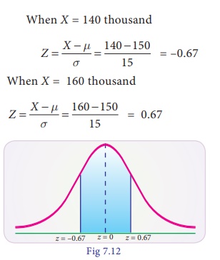
P(–0.67 < Z < 0.67) = P(–0.67 < Z < 0) + P(0 < Z < 0.67)

= P(0 < Z < 0.67) + P(0 < Z < 0.67)

= 2 P(0 < Z < < 0.67)

= 2 × 0.2486

= 0.4972

Therefore, the number of branches having sales between Rs.140 thousand and Rs.160 thousand = 550 × 0.4972 = 273

Example 7.24

Assume the mean height of children to be 69.25 cm with a variance of 10.8 cm. How many children in a school of 1,200 would you expect to be over 74 cm tall?

Solution :

Let the distribution of heights be normally distributed with mean mean 68.22 and standard deviation = 3.286

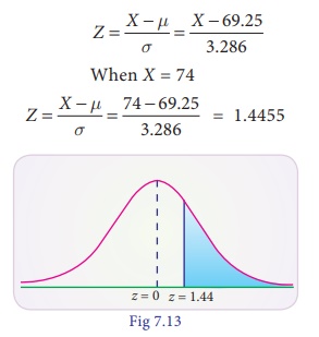
Now P(Z > 74) = P(Z > 1.44)

= 0.5 – 0.4251

= 0.0749

Expected number of children to be over 74 cm out of 1200 children

= 1200 × 0.0749 ≈ 90 children

Example 7.25

The marks obtained in a certain exam follow normal distribution with mean 45 and SD 10. If 1,300 students appeared at the examination, calculate the number of students scoring (i) less than 35 marks and (ii) more than 65 marks.

Solution :

Let X be the normal variate showing the score of the candidate with mean 45 and standard deviation 10.

(i) less than 35 marks

When X = 35

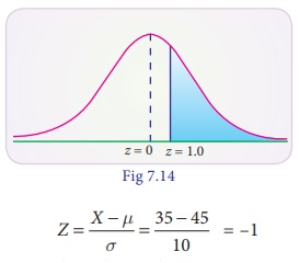
P(X < 35) = P(Z < –1)

P(Z > 1) = 0.5 – P(0 < Z < 1)

= 0.5 – 0.3413

= 0.1587

Expected number of students scoring less than 35 marks are 0.1587 × 1300

= 206

(ii) more than 65 marks

When X = 65

P(X > 65) = P(Z > 2.0)

= 0.5 – P(0 < Z < 2.0)

= 0.5 – 0.4772

= 0.0228

Expected number of students scoring more than 65 marks are 0.0228 x 1300

= 30

Example 7.26

900 light bulbs with a mean life of 125 days are installed in a new factory. Their length of life is normally distributed with a standard deviation of 18 days. What is the expected number of bulbs expire in less than 95 days?

Solution :

Let X be the normal variate of life of light bulbs with mean 125 and standard deviation 18.

(i) less than 95 days

When X = 95

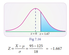
P(X < 95) = P(Z < –1.667)

= P(Z > 1.667)

= 0.5 – P(0 < Z < 1.67)

= 0.5 – 0.4525

= 0.0475

No. of bulbs expected to expire in less than 95 days out of 900 bulbs

900 × .0475 = 43 bulbs

Example 7.27

Assume that the mean height of soldiers is 69.25 inches with a variance of 9.8 inches. How many soldiers in a regiment of 6,000 would you expect to be over 6 feet tall?

Solution :

Let X be the height of soldiers follows normal distribution with mean 69.25 inches and standard deviation 3.13. then the soldiers over 6 feet tall (6ft × 12= 72 inches)

The standard normal variate

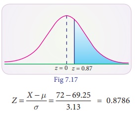
P(X > 72) = P(Z > 0.8786) = 0.5 – P(0 < Z < 0.88) = 0.5 – 0.3106 = 0.1894

Number of soldiers expected to be over 6 feet tall in 6000 are

6000 × 0.1894 =1136

Example 7.28

A bank manager has observed that the length of time the customers have to wait for being attended by the teller is normally distributed with mean time of 5 minutes and standard deviation of 0.6 minutes. Find the probability that a customer has to wait

(i) for less than 6 minutes

(ii) between 3.5 and 6.5 minutes

Solution :

Let X be the waiting time of a customer in the queue and it is normally distributed with mean 5 and SD 0.7.

(i) for less than 6 minutes

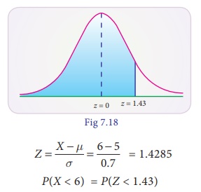
= 0.5 + 0.4236

= 0.9236

(ii) between 3.5 and 6.5 minutes

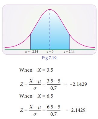
P(3.5 < X < 6.5)

= P (–2.1429 < Z < 2.1429)

= P(0 < Z < 2.1429) + P(0 < Z < 2.1429)

= 2 P(0 < Z < 2.1429)

= 2 × .4838

= 0.9676

Example 7.29

A sample of 125 dry battery cells tested to find the length of life produced the following resultd with mean 12 and sd 3 hours. Assuming that the data to be normal distributed , what percentage of battery cells are expected to have life

(i) more than 13 hours

(ii) less than 5 hours

(iii) between 9 and 14 hours

Solution :

Let X denote the length of life of dry battery cells follows normal distribution with mean 12 and sd 3 hours

(i) more than 13 hours

P(X > 13)

When X = 13

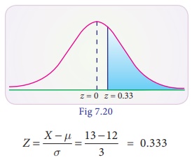
P(X > 13) = P(Z>0.333) = 0.5 – 0.1293 = 0.3707

The expected battery cells life to have more than 13 hours is

125 × 0.3707 =46.34%

(ii) less than 5 hours

P(X < 5)

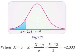
P(X < 5) = P(Z < –2.333) = P(Z > 2.333)

= 0.5 – 0.4901 = 0.0099

The expected battery cells life to have more than 13 hours is 125 × 0.0099 =1.23%

(iii) between 9 and 14 hours

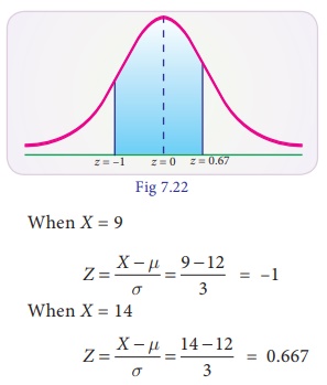
P(9 < X < 14) = P(–1 < Z < 0.667)

= P(0 < Z < 1) + P(0 < Z < 0.667)

= 0.3413 + 0.2486

= 0.5899

The expected battery cells life to have more than 13 hours is 125 x 0.5899 =73.73%

Example 7.30

Weights of fish caught by a traveler are approximately normally distributed with a mean weight of 2.25 kg and a standard deviation of 0.25 kg. What percentage of fish weigh less than 2 kg?

Solution :

We are given mean μ = 2.25 and standard deviation σ = 0.25. Probability that weight of fish is less than 2 kg is P(X < 2.0)

When x = 20

Z = [X − µ] / σ  = [2.0 − 2.25] / 0.25 = P(Z< -1.0) = P(Z > 1.0)

0.5 – 0.3413 = 0.1587

Therefore 15.87% of fishes weigh less than 2 kg.

Example 7.31

The average daily procurement of milk by village society in 800 litres with a standard deviation of 100 litres. Find out proportion of societies procuring milk between 800 litres to 1000 litres per day.

Solution :

We are given mean μ = 800 and standard deviation σ = 100 . Probability that the procurement of milk between 800 litres to 1000 litres per day is

P(800 < X < 1000)

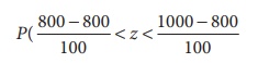
P(0 < Z < 2) = 0.4772 (table value)

Therefore 47.75 percent of societies procure milk between 800 litres to 1000 litres per day.