Introduction to Deductive Databases

Introduction to Deductive Databases

1. Overview of Deductive Databases

In a deductive database system we typically specify rules through a declarative language—a language in which we specify what to achieve rather than how to achieve it. An inference engine (or deduction mechanism) within the system can deduce new facts from the database by interpreting these rules. The model used for deductive databases is closely related to the relational data model, and particularly to the domain relational calculus formalism (see Section 6.6). It is also related to the field of logic programming and theProlog language. The deductive database work based on logic has used Prolog as a starting point. A variation of Prolog calledDatalog is used to define rules declaratively in conjunction with an existing set of relations, which are themselves treated as literals in the language. Although the language structure of Datalog resembles that of Prolog, its operational semantics—that is, how a Datalog program is executed—is still different.

A deductive database uses two main types of specifications: facts and rules. Facts are specified in a manner similar to the way relations are specified, except that it is not necessary to include the attribute names. Recall that a tuple in a relation describes some real-world fact whose meaning is partly determined by the attribute names. In a deductive database, the meaning of an attribute value in a tuple is determined solely by its position within the tuple. Rules are somewhat similar to relational views. They specify virtual relations that are not actually stored but that can be formed from the facts by applying inference mechanisms based on the rule specifications. The main difference between rules and views is that rules may involve recursion and hence may yield virtual relations that cannot be defined in terms of basic relational views.

The evaluation of Prolog programs is based on a technique called backward chaining, which involves a top-down evaluation of goals. In the deductive databases that use Datalog, attention has been devoted to handling large volumes of data stored in a relational database. Hence, evaluation techniques have been devised that resemble those for a bottom-up evaluation. Prolog suffers from the limitation that the order of specification of facts and rules is significant in evaluation; moreover, the order of literals (defined in Section 26.5.3) within a rule is significant. The execution techniques for Datalog programs attempt to circumvent these problems.

2. Prolog/Datalog Notation

The notation used in Prolog/Datalog is based on providing predicates with unique names. A predicate has an implicit meaning, which is suggested by the predicate name, and a fixed number of arguments. If the arguments are all constant values, the predicate simply states that a certain fact is true. If, on the other hand, the predicate has variables as arguments, it is either considered as a query or as part of a rule or constraint. In our discussion, we adopt the Prolog convention that all constant

values in a predicate are either numeric or character strings; they are represented as identifiers (or names) that start with a lowercase letter, whereas variable names always start with an uppercase letter.

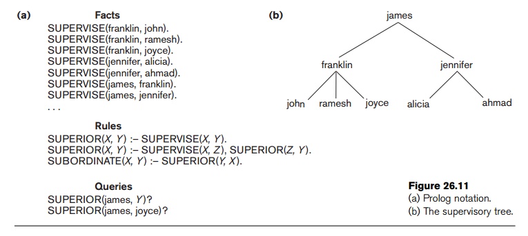
Consider the example shown in Figure 26.11, which is based on the relational data-base in Figure 3.6, but in a much simplified form. There are three predicate names: supervise, superior, and subordinate. The SUPERVISE predicate is defined via a set of facts, each of which has two arguments: a supervisor name, followed by the name of a direct supervisee (subordinate) of that supervisor. These facts correspond to the actual data that is stored in the database, and they can be considered as constituting a set of tuples in a relationSUPERVISE with two attributes whose schema is

SUPERVISE(Supervisor, Supervisee)

Thus, SUPERVISE(X, Y ) states the fact that X supervises Y. Notice the omission of the attribute names in the Prolog notation. Attribute names are only represented by virtue of the position of each argument in a predicate: the first argument represents the supervisor, and the second argument represents a direct subordinate.

The other two predicate names are defined by rules. The main contributions of deductive databases are the ability to specify recursive rules and to provide a frame-work for inferring new information based on the specified rules. A rule is of the form head :– body, where :– is read as if and only if. A rule usually has a single predicate to the left of the :– symbol—called the head or left-hand side(LHS) or conclusion of the rule—and one or more predicates to the right of the :– symbol— called the body or right-hand side(RHS) or premise(s) of the rule. A predicate with constants as arguments is said to be ground; we also refer to it as an instantiated predicate. The arguments of the predicates that appear in a rule typically include a number of variable symbols, although predicates can also contain constants as arguments. A rule specifies that, if a particular assignment or binding of constant values to the variables in the body (RHS predicates) makes all the RHS predicates true, it also makes the head (LHS predicate) true by using the same assignment of constant values to variables. Hence, a rule provides us with a way of generating new facts that are instantiations of the head of the rule. These new facts are based on facts that already exist, corresponding to the instantiations (or bind-ings) of predicates in the body of the rule. Notice that by listing multiple predicates in the body of a rule we implicitly apply the logical AND operator to these predicates. Hence, the commas between the RHS predicates may be read as meaning and.

Consider the definition of the predicate SUPERIOR in Figure 26.11, whose first argument is an employee name and whose second argument is an employee who is either a direct or an indirect subordinate of the first employee. By indirect subordinate, we mean the subordinate of some subordinate down to any number of levels. Thus SUPERIOR(X, Y ) stands for the fact that X is a superior of Ythrough direct or indirect supervision. We can write two rules that together specify the meaning of the new predicate. The first rule under Rules in the figure states that for every value of X and Y, if SUPERVISE(X, Y)—the rule body—is true, then SUPERIOR(X, Y )—the rule head—is also true, since Y would be a direct subordinate of X (at one level down). This rule can be used to generate all direct superior/subordinate relation-ships from the facts that define the SUPERVISE predicate. The second recursive rule states that ifSUPERVISE(X, Z) and SUPERIOR(Z, Y ) are both true, then SUPERIOR(X, Y) is also true. This is an example of a recursive rule, where one of the rule body predicates in the RHS is the same as the rule head predicate in the LHS. In general, the rule body defines a number of premises such that if they are all true, we can deduce that the conclusion in the rule head is also true. Notice that if we have two (or more) rules with the same head (LHS predicate), it is equivalent to saying that the predicate is true (that is, that it can be instantiated) if either one of the bodies is true; hence, it is equivalent to a logical OR operation. For example, if we have two rules X:– Y and X :– Z, they are equivalent to a rule X :– Y OR Z. The latter form is not used in deductive systems, however, because it is not in the stan-dard form of rule, called a Horn clause, as we discuss in Section 26.5.4.

A Prolog system contains a number of built-in predicates that the system can interpret directly. These typically include the equality comparison operator =(X, Y), which returns true if X and Y are identical and can also be written as X=Y by using the standard infix notation. Other comparison operators for numbers, such as <, <=, >, and >=, can be treated as binary predicates. Arithmetic functions such as +, –, *, and / can be used as arguments in predicates in Prolog. In contrast, Datalog (in its basic form) does not allow functions such as arithmetic operations as arguments; indeed, this is one of the main differences between Prolog and Datalog. However, extensions to Datalog have been proposed that do include functions.

A query typically involves a predicate symbol with some variable arguments, and its meaning (or answer) is to deduce all the different constant combinations that, when bound (assigned) to the variables, can make the predicate true. For example, the first query in Figure 26.11 requests the names of all subordinates of james at any level. A different type of query, which has only constant symbols as arguments, returns either a true or a false result, depending on whether the arguments provided can be deduced from the facts and rules. For example, the second query in Figure 26.11 returns true, since SUPERIOR(james, joyce) can be deduced.

3. Datalog Notation

In Datalog, as in other logic-based languages, a program is built from basic objects called atomic formulas. It is customary to define the syntax of logic-based languages by describing the syntax of atomic formulas and identifying how they can be combined to form a program. In Datalog, atomic formulas are literals of the form p(a1, a2, ..., an), where p is the predicate name and n is the number of arguments for predicate p. Different predicate symbols can have different numbers of arguments, and the number of arguments n of predicate p is sometimes called the arity or degree of p. The arguments can be either constant values or variable names. Asmentioned earlier, we use the convention that constant values either are numeric or start with a lowercase character, whereas variable names always start with an uppercase character.

A number of built-in predicates are included in Datalog, which can also be used to construct atomic formulas. The built-in predicates are of two main types: the binary comparison predicates < (less), <= (less_or_equal), > (greater), and >= (greater_or_equal) over ordered domains; and the comparison predicates = (equal) and /= (not_equal) over ordered or unordered domains. These can be used as binary predicates with the same functional syntax as other predicates—for example, by writing less(X, 3)—or they can be specified by using the customary infix notation X<3. Note that because the domains of these predicates are potentially infinite, they should be used with care in rule definitions. For example, the predicate greater(X, 3), if used alone, generates an infinite set of values for X that satisfy the predicate (all integer numbers greater than 3).

A literal is either an atomic formula as defined earlier—called a positive literal—or an atomic formula preceded by not. The latter is a negated atomic formula, called a negative literal. Datalog programs can be considered to be a subset of the predicate calculus formulas, which are somewhat similar to the formulas of the domain relational calculus (see Section 6.7). In Datalog, however, these formulas are first con-verted into what is known as clausal form before they are expressed in Datalog, and only formulas given in a restricted clausal form, called Horn clauses, can be used in Datalog.

4. Clausal Form and Horn Clauses

Recall from Section 6.6 that a formula in the relational calculus is a condition that includes predicates called atoms (based on relation names). Additionally, a formula can have quantifiers—namely, the universal quantifier (for all) and the existential quantifier (there exists). In clausal form, a formula must be transformed into another formula with the following characteristics:

·        All variables in the formula are universally quantified. Hence, it is not necessary to include the universal quantifiers (for all) explicitly; the quantifiers are removed, and all variables in the formula are implicitly quantified by the universal quantifier.

·        In clausal form, the formula is made up of a number of clauses, where each clause is composed of a number of literals connected by OR logical connectives only. Hence, each clause is a disjunction of literals.

·        The clauses themselves are connected by AND logical connectives only, to form a formula. Hence, the clausal form of a formula is a conjunction of clauses.

It can be shown that any formula can be converted into clausal form. For our purposes, we are mainly interested in the form of the individual clauses, each of which is a disjunction of literals. Recall that literals can be positive literals or negative literals. Consider a clause of the form:

This clause has n negative literals and m positive literals. Such a clause can be trans-formed into the following equivalent logical formula:

where ⇒ is the implies symbol. The formulas (1) and (2) are equivalent, meaning that their truth values are always the same. This is the case because if all the Pi liter-als (i = 1, 2, ..., n) are true, the formula (2) is true only if at least one of the Qi’s is true, which is the meaning of the ⇒ (implies) symbol. For formula (1), if all the Pi literals (i = 1, 2, ..., n) are true, their negations are all false; so in this case formula

(1) is true only if at least one of the Qi’s is true. In Datalog, rules are expressed as a restricted form of clauses called Horn clauses, in which a clause can contain at most one positive literal. Hence, a Horn clause is either of the form

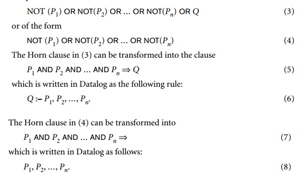
A Datalog rule, as in (6), is hence a Horn clause, and its meaning, based on formula (5), is that if the predicates P1 AND P2 AND ...AND Pn are all true for a particular binding to their variable arguments, then Q is also true and can hence be inferred. The Datalog expression (8) can be considered as an integrity constraint, where all the predicates must be true to satisfy the query.

In general, a query in Datalog consists of two components:

        A Datalog program, which is a finite set of rules

        A literal P(X1, X2, ..., Xn), where each Xi is a variable or a constant

A Prolog or Datalog system has an internal inference engine that can be used to process and compute the results of such queries. Prolog inference engines typically return one result to the query (that is, one set of values for the variables in the query) at a time and must be prompted to return additional results. On the con-trary, Datalog returns results set-at-a-time.

5. Interpretations of Rules

There are two main alternatives for interpreting the theoretical meaning of rules: proof-theoretic and model-theoretic. In practical systems, the inference mechanism within a system defines the exact interpretation, which may not coincide with either of the two theoretical interpretations. The inference mechanism is a computational procedure and hence provides a computational interpretation of the meaning of rules. In this section, first we discuss the two theoretical interpretations. Then we briefly discuss inference mechanisms as a way of defining the meaning of rules.

In the proof-theoretic interpretation of rules, we consider the facts and rules to be true statements, or axioms. Ground axiomscontain no variables. The facts are ground axioms that are given to be true. Rules are called deductive axioms, since they can be used to deduce new facts. The deductive axioms can be used to con-struct proofs that derive new facts from existing facts. For example, Figure 26.12 shows how to prove the fact SUPERIOR(james, ahmad) from the rules and facts

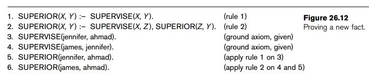
given in Figure 26.11. The proof-theoretic interpretation gives us a procedural or computational approach for computing an answer to the Datalog query. The process of proving whether a certain fact (theorem) holds is known as theorem proving.

The second type of interpretation is called the model-theoretic interpretation. Here, given a finite or an infinite domain of constant values,33 we assign to a predicate every possible combination of values as arguments. We must then determine whether the predicate is true or false. In general, it is sufficient to specify the combinations of arguments that make the predicate true, and to state that all other combi-nations make the predicate false. If this is done for every predicate, it is called an interpretation of the set of predicates. For example, consider the interpretation shown in Figure 26.13 for the predicates SUPERVISE and SUPERIOR. This interpretation assigns a truth value (true or false) to every possible combination of argument values (from a finite domain) for the two predicates.

An interpretation is called a model for a specific set of rules if those rules are always true under that interpretation; that is, for any values assigned to the variables in the rules, the head of the rules is true when we substitute the truth values assigned to the predicates in the body of the rule by that interpretation. Hence, whenever a particular substitution (binding) to the variables in the rules is applied, if all the predicates in the body of a rule are true under the interpretation, the predicate in the head of the rule must also be true. The interpretation shown in Figure 26.13 is a model for the two rules shown, since it can never cause the rules to be violated. Notice that a rule is violated if a particular binding of constants to the variables makes all the predicates in the rule body true but makes the predicate in the rule head false. For example, if SUPERVISE(a, b) and SUPERIOR(b, c) are both true under some interpretation, but SUPERIOR(a, c) is not true, the interpretation can-not be a model for the recursive rule:

SUPERIOR(X, Y) :– SUPERVISE(X, Z), SUPERIOR(Z, Y)

In the model-theoretic approach, the meaning of the rules is established by providing a model for these rules. A model is called aminimal model for a set of rules if we cannot change any fact from true to false and still get a model for these rules. For example, consider the interpretation in Figure 26.13, and assume that the SUPERVISE predicate is defined by a set of known facts, whereas the SUPERIOR predicate is defined as an interpretation (model) for the rules. Suppose that we add the predicate SUPERIOR(james, bob) to the true predicates. This remains a model for the rules shown, but it is not a minimal model, since changing the truth value ofSUPERIOR(james,bob) from true to false still provides us with a model for the rules. The model shown in Figure 26.13 is the minimal model for the set of facts that are defined by the SUPERVISE predicate.

In general, the minimal model that corresponds to a given set of facts in the model-theoretic interpretation should be the same as the facts generated by the proof

Rules         

SUPERIOR(X, Y ) :–  SUPERVISE(X, Y ).                 

SUPERIOR(X, Y ) :–  SUPERVISE(X, Z ), SUPERIOR(Z, Y ).               

Interpretation                

Known Facts:               

SUPERVISE(franklin, john) is true.          

SUPERVISE(franklin, ramesh) is true.               

SUPERVISE(franklin, joyce) is true.                  

SUPERVISE(jennifer, alicia) is true.         

SUPERVISE(jennifer, ahmad) is true.                

SUPERVISE(james, franklin) is true.                 

SUPERVISE(james, jennifer) is true.                  

SUPERVISE(X, Y ) is false for all other possible (X, Y ) combinations            

Derived Facts:               

SUPERIOR(franklin, john) is true.            

SUPERIOR(franklin, ramesh) is true.                 

SUPERIOR(franklin, joyce) is true.           

SUPERIOR(jennifer, alicia) is true.           

SUPERIOR(jennifer, ahmad) is true.                  

SUPERIOR(james, franklin) is true.          

SUPERIOR(james, jennifer) is true.          

SUPERIOR(james, john) is true.               

SUPERIOR(james, ramesh) is true.           

SUPERIOR(james, joyce) is true.              

SUPERIOR(james, alicia) is true.

SUPERIOR(james, ahmad) is true.  

SUPERIOR(X, Y ) is false for all other possible (X, Y ) combinations     

Figure 26.13 An interpretation that is a minimal model.

theoretic interpretation for the same original set of ground and deductive axioms. However, this is generally true only for rules with a simple structure. Once we allow negation in the specification of rules, the correspondence between interpretations does not hold. In fact, with negation, numerous minimal models are possible for a given set of facts.

A third approach to interpreting the meaning of rules involves defining an inference mechanism that is used by the system to deduce facts from the rules. This inference mechanism would define a computational interpretation to the meaning of the rules. The Prolog logic programming language uses its inference mechanism to define the meaning of the rules and facts in a Prolog program. Not all Prolog pro-grams correspond to the proof-theoretic or model-theoretic interpretations; it depends on the type of rules in the program. However, for many simple Prolog pro-grams, the Prolog inference mechanism infers the facts that correspond either to the proof-theoretic interpretation or to a minimal model under the model-theoretic interpretation.

6. Datalog Programs and Their Safety

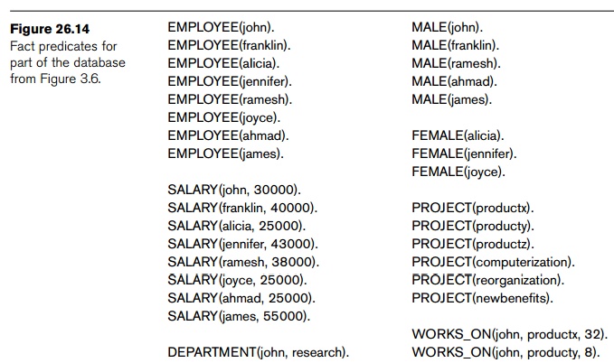
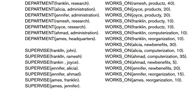
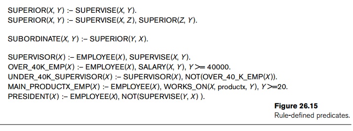
There are two main methods of defining the truth values of predicates in actual Datalog programs. Fact-defined predicates (orrelations) are defined by listing all the combinations of values (the tuples) that make the predicate true. These correspond to base relations whose contents are stored in a database system. Figure 26.14 shows the fact-defined predicates EMPLOYEE, MALE,FEMALE, DEPARTMENT, SUPERVISE, PROJECT, and WORKS_ON, which correspond to part of the relational database shown in Figure 3.6. Rule-defined predicates (or views) are defined by being the head (LHS) of one or more Datalog rules; they correspond to virtual rela tions whose contents can be inferred by the inference engine. Figure 26.15 shows a number of rule-defined predicates

A program or a rule is said to be safe if it generates a finite set of facts. The general theoretical problem of determining whether a set of rules is safe is undecidable. However, one can determine the safety of restricted forms of rules. For example, the rules shown in Figure 26.16 are safe. One situation where we get unsafe rules that can generate an infinite number of facts arises when one of the variables in the rule can range over an infinite domain of values, and that variable is not limited to ranging over a finite relation. For example, consider the following rule:

BIG_SALARY(Y ) :– Y>60000

Here, we can get an infinite result if Y ranges over all possible integers. But suppose that we change the rule as follows:

BIG_SALARY(Y ) :– EMPLOYEE(X), Salary(X, Y ), Y>60000

In the second rule, the result is not infinite, since the values that Y can be bound to are now restricted to values that are the salary of some employee in the database— presumably, a finite set of values. We can also rewrite the rule as follows:

BIG_SALARY(Y ) :– Y>60000, EMPLOYEE(X ), Salary(X, Y )

In this case, the rule is still theoretically safe. However, in Prolog or any other system that uses a top-down, depth-first inference mechanism, the rule creates an infinite loop, since we first search for a value for Y and then check whether it is a salary of an employee. The result is generation of an infinite number of Y values, even though these, after a certain point, cannot lead to a set of true RHS predicates. One definition of Datalog considers both rules to be safe, since it does not depend on a particular inference mechanism. Nonetheless, it is generally advisable to write such a rule in the safest form, with the predicates that restrict possible bindings of variables placed first. As another example of an unsafe rule, consider the following rule:

HAS_SOMETHING(X, Y ) :– EMPLOYEE(X )

REL_ONE(A, B, C ).

REL_TWO(D, E, F ).

REL_THREE(G, H, I, J ).

SELECT_ONE_A_EQ_C(X, Y, Z ) :– REL_ONE(C, Y, Z ).

SELECT_ONE_B_LESS_5(X, Y, Z ) :– REL_ONE(X, Y, Z ), Y< 5.

SELECT_ONE_A_EQ_C_AND_B_LESS_5(X, Y, Z ) :– REL_ONE(C, Y, Z ), Y<5

SELECT_ONE_A_EQ_C_OR_B_LESS_5(X, Y, Z ) :– REL_ONE(C, Y, Z ).

SELECT_ONE_A_EQ_C_OR_B_LESS_5(X, Y, Z ) :– REL_ONE(X, Y, Z ), Y<5.

PROJECT_THREE_ON_G_H(W, X ) :–  REL_THREE(W, X, Y, Z ).

UNION_ONE_TWO(X, Y, Z ) :–  REL_ONE(X, Y, Z ).

UNION_ONE_TWO(X, Y, Z ) :–  REL_TWO(X, Y, Z ).

INTERSECT_ONE_TWO(X, Y, Z ) :–  REL_ONE(X, Y, Z ), REL_TWO(X, Y, Z ).

DIFFERENCE_TWO_ONE(X, Y, Z ) :–  REL_TWO(X, Y, Z ) NOT(REL_ONE(X, Y, Z ).

CART  PROD _ONE_THREE(T, U, V, W, X, Y, Z ) :–

REL_ONE(T, U, V), REL_THREE(W, X, Y, Z ).

NATURAL_JOIN_ONE_THREE_C_EQ_G(U, V, W, X, Y, Z ) :–

REL_ONE(U, V, W ), REL_THREE(W, X, Y, Z ).

Figure 26.16

Predicates for illustrating relational operations.

Here, an infinite number of Y values can again be generated, since the variable Y appears only in the head of the rule and hence is not limited to a finite set of values. To define safe rules more formally, we use the concept of a limited variable. A variable X is limited in a rule if (1) it appears in a regular (not built-in) predicate in the body of the rule; (2) it appears in a predicate of the form X=c or c=Xor (c1<<=X and X<=c2) in the rule body, where c, c1, and c2 are constant values; or (3) it appears in a predicate of the form X=Y orY=X in the rule body, where Y is a limited vari-able. A rule is said to be safe if all its variables are limited.

7. Use of Relational Operations

It is straightforward to specify many operations of the relational algebra in the form of Datalog rules that define the result of applying these operations on the database relations (fact predicates). This means that relational queries and views can easily be specified in Datalog. The additional power that Datalog provides is in the specification of recursive queries, and views based on recursive queries. In this section, we show how some of the standard relational operations can be specified as Datalog rules. Our examples will use the base relations (fact-defined predicates) REL_ONE, REL_TWO, and REL_THREE, whose schemas are shown in Figure 26.16. In Datalog, we do not need to specify the attribute names as in Figure 26.16; rather, the arity (degree) of each predicate is the important aspect. In a practical system, the domain (data type) of each attribute is also important for operations such as UNION,INTERSECTION, and JOIN, and we assume that the attribute types are compatible for the various operations, as discussed in Chapter 3.

Figure 26.16 illustrates a number of basic relational operations. Notice that if the Datalog model is based on the relational model and hence assumes that predicates (fact relations and query results) specify sets of tuples, duplicate tuples in the same predicate are automatically eliminated. This may or may not be true, depending on the Datalog inference engine. However, it is definitely not the case in Prolog, so any of the rules in Figure 26.16 that involve duplicate elimination are not correct for Prolog. For example, if we want to specify Prolog rules for the UNION operation with duplicate elimination, we must rewrite them as follows:

UNION_ONE_TWO(X, Y, Z) :– REL_ONE(X, Y, Z).

UNION_ONE_TWO(X, Y, Z) :– REL_TWO(X, Y, Z), NOT(REL_ONE(X, Y, Z)).

However, the rules shown in Figure 26.16 should work for Datalog, if duplicates are automatically eliminated. Similarly, the rules for the PROJECT operation shown in Figure 26.16 should work for Datalog in this case, but they are not correct for Prolog, since duplicates would appear in the latter case.

8. Evaluation of Nonrecursive Datalog Queries

In order to use Datalog as a deductive database system, it is appropriate to define an inference mechanism based on relational database query processing concepts. The inherent strategy involves a bottom-up evaluation, starting with base relations; the order of operations is kept flexible and subject to query optimization. In this section we discuss an inference mechanism based on relational operations that can be applied to nonrecursive Datalog queries. We use the fact and rule base shown in Figures 26.14 and 26.15 to illustrate our discussion.

If a query involves only fact-defined predicates, the inference becomes one of searching among the facts for the query result. For example, a query such as

DEPARTMENT(X, Research)?

is a selection of all employee names X who work for the Research department. In relational algebra, it is the query:

π$1 (σ$2 = “Research” (DEPARTMENT))

which can be answered by searching through the fact-defined predicate department(X,Y ). The query involves relational SELECTand PROJECT operations on a base relation, and it can be handled by the database query processing and opti-mization techniques discussed in Chapter 19.

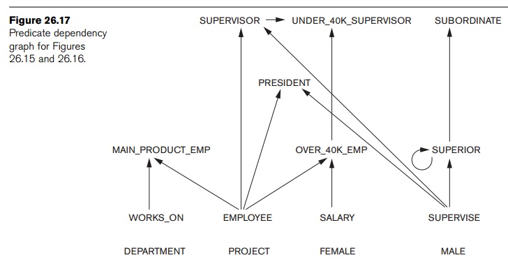
When a query involves rule-defined predicates, the inference mechanism must compute the result based on the rule definitions. If a query is nonrecursive and involves a predicate p that appears as the head of a rule p :– p1, p2, ..., pn, the strategy is first to compute the relations corresponding to p1, p2, ..., pn and then to compute the relation corresponding to p. It is useful to keep track of the dependency among the predicates of a deductive database in a predicate dependency graph. Figure 26.17 shows the graph for the fact and rule predicates shown in Figures 26.14 and 26.15. The dependency graph contains a node for each predicate. Whenever a predicate A is specified in the body (RHS) of a rule, and the head (LHS) of that rule is the predicate B, we say that B depends on A, and we draw a directed edge from A to B. This indicates that in order to compute the facts for the predicate B (the rule head), we must first compute the facts for all the predicates A in the rule body. If the dependency graph has no cycles, we call the rule setnonrecursive. If there is at least one cycle, we call the rule set recursive. In Figure 26.17, there is one recursively defined predicate—namely, SUPERIOR—which has a recursive edge pointing back to itself. Additionally, because the predicate subordinate depends onSUPERIOR, it also requires recursion in computing its result.

A query that includes only nonrecursive predicates is called a nonrecursive query. In this section we discuss only inference mechanisms for nonrecursive queries. In Figure 26.17, any query that does not involve the predicates SUBORDINATE orSUPERIOR is nonrecursive. In the predicate dependency graph, the nodes corresponding to fact-defined predicates do not have any incoming edges, since all fact-defined predicates have their facts stored in a database relation. The contents of a fact-defined predicate can be computed by directly retrieving the tuples in the cor-responding database relation.

The main function of an inference mechanism is to compute the facts that correspond to query predicates. This can be accomplished by generating a relational expression involving relational operators as SELECT, PROJECT, JOIN, UNION, and SET DIFFERENCE (with appropriate provision for dealing with safety issues) that, when executed, provides the query result. The query can then be executed by utilizing the internal query processing and optimization operations of a relational data-base management system. Whenever the inference mechanism needs to compute the fact set corresponding to a nonrecursive rule-defined predicate p, it first locates all the rules that have p as their head. The idea is to compute the fact set for each such rule and then to apply the UNIONoperation to the results, since UNION corresponds to a logical OR operation. The dependency graph indicates all predicates q on which each p depends, and since we assume that the predicate is nonrecursive, we can always determine a partial order among such predicates q. Before computing the fact set for p, first we compute the fact sets for all predicates q on which p depends, based on their partial order. For example, if a query involves the predicate UNDER_40K_SUPERVISOR,  we     must                 first  compute      both                                      SUPERVISOR       and OVER_40K_EMP. Since the latter two depend only on the fact-defined predicates EMPLOYEE, SALARY, and SUPERVISE, they can be computed directly from the stored database relations.

This concludes our introduction to deductive databases. Additional material may be found at the book’s Website, where the complete Chapter 25 from the third edition is available. This includes a discussion on algorithms for recursive query processing. We have included an extensive bibliography of work in deductive databases, recursive query processing, magic sets, combination of relational databases with deductive rules, and GLUE-NAIL! System at the end of this chapter.