Examples of a Bar Finite Element

EXAMPLES OF A BAR FINITE ELEMENT

The finite element method can be used to solve a variety of problem types in engineering, mathematics and science. The three main areas are mechanics of materials, heat transfer and fluid mechanics. The one-dimensional spring element belongs to the area of mechanics of materials, since it deals with the displacements, deformations and stresses involved in a solid body subjected to external loading.

Element dimensionality:

An element can be one-dimensional, two-dimensional or three-dimensio nal. A spring element is classified as one-dimensional.

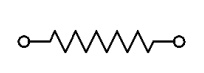
Geometric shape of the element

The geometric shape of element can be represented as a line, area, or volume. The one-dimensional spring element is defi ned geometrically as:

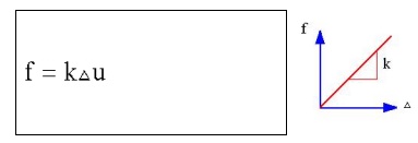
Spring law

The spring is assumed to b e linear. Force (f) is directly proportional to deformation (Δ) via the spring constant k, i.e.

Types of degrees of freedom per n ode

Degrees of freedom are displacements and/or rotations that are associated with a node. A one-dimensional spring element has two translational degrees of freedom, whi ch include, an axial (horizontal) displacement (u) at ea ch node.

Element formulation

There are various ways to mathematically formulate an element. The simplest and limited approach is the direct method. More mathematically complex and general ap proaches are energy (variation) and weighted residual methods.

The direct method uses the fundamentals of equilibrium, compatibility and spring law from a sophomore level mechanics of material course. We will use the direct method to formulate the one-dimensional spring element because it is simple and based on a physical approach.

The direct method is an excellent setting for becoming familiar with such basis concepts of linear algebra, stiffness, degrees of freedom, etc., before using the mathematical formulation approaches as energy or weighted residuals.

Assumptions

Spring deformation

The spring law is a linear force-deformation as follows:

f = k

f - Spring Force (units: force)

k - Spring Constant (units: force/length)

- Spring Deformation (units: length)

Spring Behaviour:

A spring behaves the same in tension and compression.

Spring Stiffness:

Spring stiffness k is always positive, i.e., k>0, for a physical linear system.

Nodal Force Direction:

Loading is uniaxial, i.e., the resultant force is along the element. Spring has no resistance to lateral force.

Weightless Member:

Element has no mass (weightless).

Node Location:

The geometric location of nodes I and J cannot coincide, i.e., xi ≠ xj. The length of the element is only used to visually see the spring.

A column of KE is a vector of nodal loads that must be applied to an element to sustain a deformed state in which responding nodal DOF has unit value and all other nodal DOF are zero. In other words, a column of KE represents an equilibrium problem.

Example, uI = 1, uJ = 0.

Spring element has one rigid body mode.

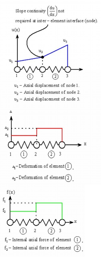
Inter-Element Axial Displacement

The axial displacement (u ) is continuous through the assembled mesh a nd is described by a linear polynomial within each el ement. Each element in the mesh may be described by a different linear polynomial, depending on t he spring rate (k), external loading, and constraints on the element.

Inter-Element Deformation

The deformation (Δ) is pi ecewise constant through the assembled mesh and is described by a constant within each element. Ea ch element in the mesh may be described by a different constant, depending on the spring constant ( k), external loading, and constraints on the elem ent.

Inter-Element Internal Axial Forc e

The internal axial force (f) is piecewise continuous through the assembled mesh and is described by a constant within eac h element. Each element in the mesh may be described by a different constant, depending on the spring constant, external loading, and constraints on the element.

1 Rigid Body

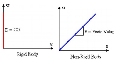
A body is considered rigi d if it does not deform when a force is applied. Consider rigid and non-rigid bars subjected to a graduually applied axial force of increasing magnitud e as shown.

The reader should note the followiing characteristics of rigid and non-rigid (flexib le) bodies:

·        Force Magnitude - Even if forces are large, a rigid body does not deform. A non-rigid body will deform even if a force is s mall. In reality, all bodies deform.

·        Failure - A rigid body does not fail under any load; while a non-rigid bod y will result either in

ductile or brittle failure w hen the applied load causes the normal stress t o exceed the breaking (fracture) stress   b of the material. Brittle failure occurs when the applied load on the non-rigid bar shown above causes the breaking strength of the bar to be exceeded.

·        Material - The material is not considered in a rigid body. Since a rigid bod y does not deform (   = 0) this is equivalent to an infinite modulus of elasticity. In contrast the modulus of elasticity

for a non-rigid material is finite, e.g., for steel, Esteel = 30 x 106 psi. (20 0 GPa). For rigid and non-rigid bars the material laws are:

Rigid Body Motion

Rigid body motion occurs when forces and/or moments are applied to an unrestrained mesh (body), resulting in motion that occurs without any deformations in the entire m esh (body). Since no strains (deformations) occur during rigid body motion, there can be no stresses developed in the mesh.

A rigid body in general can be subjected to three types of motion, w hich are translation, rotation about a fixed axis, and general motion which consists of a combination o f both translation and rotation. These three motion types are as follows:

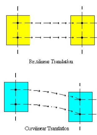
Translation - If any line segment on the body remains parallel to its original direction during the motion, it is said to be in translation. When the path of motion is along a straight line, the motion is called rectilinear translation, while a curved path is considered as a curvilinear translation. The curvilinear motion shown below is a combination of two translational motions, o ne horizontal motion and one vertical motion.

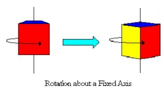
Rotation About a Fixe d Axis - If all the particles of a rigid body mov e along circular paths, except the ones which lie on the axis of rotation, it is said to be in rotation ab out a fixed axis.

General Motion - Any motion of a rigid body that consists of the combination of both translations

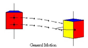
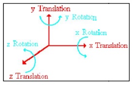
There are six rigid bo dy modes in general three-dimensional situati on; three translational along the x, y, and z axes and three rotational about x, y, and z axes. Illustratio ns of these rigid body modes are presented as follows:

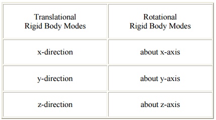
Translational Rigid Body Modes :              Rotational Rigid Body Modes

x-direction            about x-axis

y-direction            about y-axis

z-direction            about z-axis

1-D 3-NODED QUADRATIC BAR ELEMENT

Problem 6

A single 1-D 3-noded quadratic bar element has 3 nodes with local coordinates as shown in

Figure

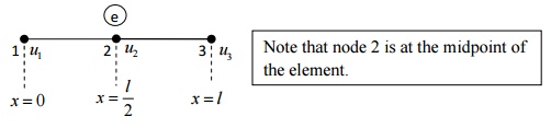
The chosen approximation function for the field variable u is u = a + bx + cx2

Let the field variable u  have values u1 , u2 and u3 at nodes 1, 2 and 3, respectively.

To find the unknowns a, b and c, we apply the boundary conditions

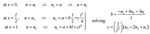
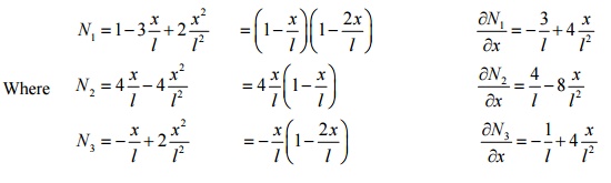
Substituting the values of a, b and c in equation (1) and collecting the coefficients of u1 , u 2  and u3

u = N1u1 + N 2 u 2 + N 3u3

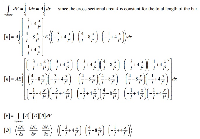
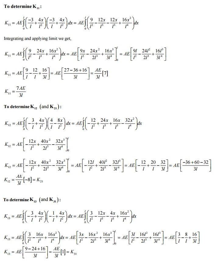
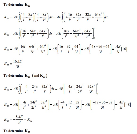
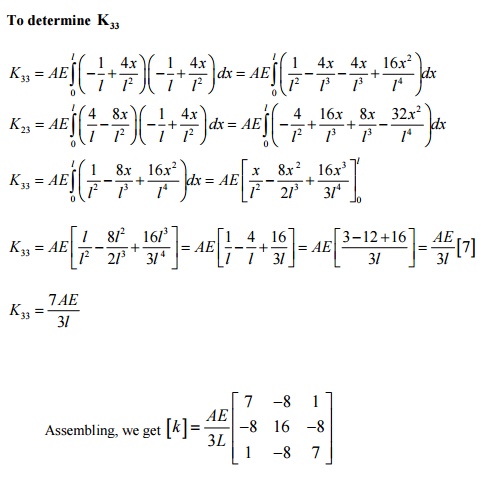
Derivation of stiffness matrix for 1-D 3-noded quadratic bar element:

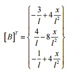
[D ] = E for a bar element (1-D case - only axial stress (s x ) and strain (e x ) exist Þ s x  = Ee x )