Datalog Implementation by BDD's

Datalog Implementation by BDD's

1 Binary Decision Diagrams

2 Transformations on BDD's

3 Representing Relations by BDD's

4 A Relational Operations as BDD Operations

5 Using BDD's for Points-to Analysis

6 Exercises for Section 12.7

Binary Decision Diagrams (BDD's) are a method for representing boolean func-tions by graphs. Since there are 2 ² " boolean functions of n variables, no repre-sentation method is going to be very succinct on all boolean functions. However, the boolean functions that appear in practice tend to have a lot of regularity. It is thus common that one can find a succinct BDD for functions that one really wants to represent.

It turns out that the boolean functions that are described by the Datalog programs that we have developed to analyze programs are no exception. While succinct BDD's representing information about a program often must be found using heuristics and/or techniques used in commercial BDD-manipulating pack-ages, the BDD approach has been quite successful in practice. In particular, it outperforms methods based on conventional database-management systems, because the latter are designed for the more irregular data patterns that appear in typical commercial data.

It is beyond the scope of this book to cover all of the BDD technology that has been developed over the years. We shall here introduce you to the BDD notation. We then suggest how one represents relational data as BDD's and how one could manipulate BDD's to reflect the operations that are performed to execute Datalog programs by algorithms such as Algorithm 12.18. Finally, we describe how to represent the exponentially many contexts in BDD's, the key to the success of the use of BDD's in context-sensitive analysis.

1. Binary Decision Diagrams

A BDD represents a boolean function by a rooted DAG. The interior nodes of the DAG are each labeled by one of the variables of the represented function. At the bottom are two leaves, one labeled 0 the other labeled 1. Each interior node has two edges to children; these edges are called "low" and "high." The low edge is associated with the case that the variable at the node has value 0, and the high edge is associated with the case where the variable has value 1.

Given a truth assignment for the variables, we can start at the root, and at each node, say a node labeled x, follow the low or high edge, depending on whether the truth value for x is 0 or 1, respectively. If we arrive at the leaf labeled 1, then the represented function is true for this truth assignment; otherwise it is false.

Example 12 . 27: In Fig. 12.31 we see a BDD. We shall see the function it represents shortly. Notice that we have labeled all the "low" edges with 0 and

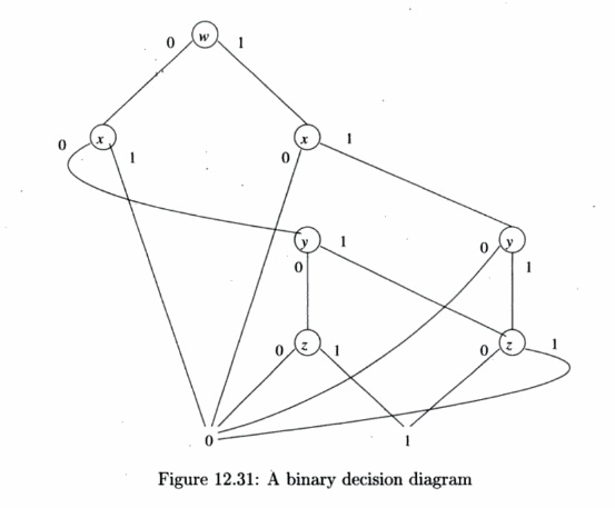
all the "high" edges by 1. Consider the truth assignment for variables wxyz that sets w = x = y = 0 and z = 1. Starting at the root, since w — 0 we take the low edge, which gets us to the leftmost of the nodes labeled x. Since x = 0, we again follow the low edge from this node, which takes us to the leftmost of the nodes labeled y. Since y = 0 we next move to the leftmost of the nodes labeled z. Now, since z = 1, we take the high edge and wind up at the leaf labeled 1. Our conclusion is that the function is true for this truth assignment.

Now, consider the truth assignment wxyz = 0101, that is, w = y = 0 and x = z = 1. We again start at the root. Since w = 0 we again move to the leftmost of the nodes labeled x. But now, since x = 1, we follow the high edge, which jumps to the 0 leaf. That is, we know not only that truth assignment 0101 makes the function false, but since we never even looked at y or z, any truth assignment of the form Qlyz will also make the function have value 0. This "short-circuiting" ability is one of the reasons BDD's tend to be succinct representations of boolean functions. •

In Fig. 12.31 the interior nodes are in ranks — each rank having nodes with a particular variable as label. Although it is not an absolute requirement, it is convenient to restrict ourselves to ordered BDD's. In an ordered BDD, there is an order x1,xi,... ,xn to the variables, and whenever there is an edge from a parent node labeled Xi to a child labeled Xj, then i < j. We shall see that it is easier to operate on ordered BDD's, and from here we assume all BDD's are ordered.

Notice also that BDD's are DAG's, not trees. Not only will the leaves 0 and 1 typically have many parents, but interior nodes also may have several parents. For example, the rightmost of the nodes labeled z in Fig. 12.31 has two parents. This combination of nodes that would result in the same decision is another reason that BDD's tend to be succinct.

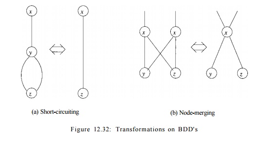
2. Transformations on BDD's

We alluded, in the discussion above, to two simplifications on BDD's that help make them more succinct:

1.            Short-Circuiting: If a node N has both its high and low edges go to the same node M, then we may eliminate N. Edges entering N go to M instead.

2.            Node-Merging: If two nodes N and M have low edges that go to the same node and also have high edges that go to the same node, then we may merge N with M. Edges entering either N or M go to the merged node.

It is also possible to run these transformations in the opposite direction. In particular, we can introduce a node along an edge from N to M. Both edges from the introduced node go to M, and the edge from TV" now goes to the introduced node. Note, however, that the variable assigned to the new node must be one of those that lies between the variables of N and M in the order. Figure 12.32 shows the two transformations schematically.

3. Representing Relations by BDD's

The relations with which we have been dealing have components that are taken frorn "domains." A domain for a component of a relation is the set of possible values that tuples can have in that component. For example, the relation pts(V, H) has the domain of all program variables for its first component and the domain of all object-creating statements for the second component. If a domain has more than 2 ^{n _ 1} possible values but no more than 2 ⁿ values, then it requires n bits or boolean variables to represent values in that domain.

A tuple in a relation may thus be viewed as a truth assignment to the variables that represent values in the domains for each of the components of the tuple. We may see a relation as a boolean function that returns the value true for all and only those truth assignments that represent tuples in the relation. An example should make these ideas clear.

Example 1 2 . 2 8 : Consider a relation r(A, B) such that the domains of both A and B are {a, b, c, d}. We shall encode a by bits 00, b by 01, c by 10, and d by 11. Let the tuples of relation r be: 

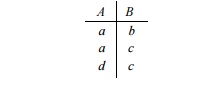
Let us use boolean variables wx to encode the first (A) component and variables yz to encode the second (B) component. Then the relation r becomes:

That is, the relation r has been converted into the boolean function that is true for the three truth-assignments wxyz = 0001, 0010, and 1110. Notice that these three sequences of bits are exactly those that label the paths from the root to the leaf 1 in Fig. 12.31. That is, the BDD in that figure represents this relation r, if the encoding described above is used. •

4. Relational Operations as BDD Operations

Now we see how to represent relations as BDD's. But to implement an algorithm like Algorithm 12.18 (incremental evaluation of Datalog programs), we need to manipulate BDD's in a way that reflects how the relations themselves are manipulated. Here are the principal operations on relations that we need to perform:

1. Initialization: We need to create a BDD that represents a single tuple of  a relation.  We'll assemble these into BDD's that represent large relations  by taking the union.  

2. Union: To take the union of relations, we take the logical OR of the boolean functions that represent the relations. This operation is needed not only to construct initial relations, but also to combine the results of several rules for the same head predicate, and to accumulate new facts into the set of old facts, as in the incremental Algorithm 12.18.

3.          Projection: When we evaluate a rule body, we need to construct the head relation that is implied by the true tuples of the body. In terms of the  BDD that represents the relation, we need to eliminate the nodes that are labeled by those boolean variables that do not represent components of the head. We may also need to rename the variables in the BDD to correspond to the boolean variables for the components of the head relation.

4. Join: To find the assignments of values to variables that make a rule body true, we need to "join" the relations corresponding to each of the subgoals. For example, suppose we have two subgoals r(A,B) k s(B, C).

The join of the relations for these subgoals is the set of (a, 6, c) triples such that (a, 6) is a tuple in the relation for r, and (6, c) is a tuple in the relation for s. We shall see that, after renaming boolean variables in BDD's so the components for the two B's agree in variable names, the operation on BDD's is similar to the logical AND, which in turn is similar to the OR operation on BDD's that implements the union.

BDD ' s for Single Tuples

To initialize a relation, we need to have a way to construct a BDD for the function that is true for a single truth assignment. Suppose the boolean variables are Xi,x2, • • • ,xn, and the truth assignment is a1a2  • • • an, where each ai is either 0 or 1. The BDD will have one node Ni for each Xi. If = 0, then the high edge from Ni leads to the leaf 0, and the low edge leads to Ni+1, or to the leaf 1 if i = n. If a» = 1, then we do the same, but the high and low edges are reversed.

This strategy gives us a BDD that checks whether each Xi has the correct value, for i = 1,2, ... , n. As soon as we find an incorrect value, we jump directly to the 0 leaf. We only wind up at the 1 leaf if all variables have their correct value.

As an example, look ahead to Fig. 12.33(b). This BDD represents the function that is true if and only if x = y = 0, i.e., the truth assignment 00.

Union

We shall give in detail an algorithm for taking the logical OR of BDD's, that is, the union of the relations represented by the BDD's.

Algorithm 1 2 . 2 9 : Union of BDD's.

INPUT : Two ordered BDD's with the same set of variables, in the same order.

OUTPUT : A BDD representing the function that is the logical OR of the two boolean functions represented by the input BDD's.

M E T H O D : We shall describe a recursive procedure for combining two BDD's. The induction is on the size of the set of variables appearing in the BDD's.

BASIS: Zero variables. The BDD's must both be leaves, labeled either 0 or 1. The output is the leaf labeled 1 if either input is 1, or the leaf labeled 0 if both are 0.

I N D U C T I O N : Suppose there are k variables, yi,y₂,... ,yu found among the two BDD's. Do the following:

1.         If necessary, use inverse short-circuiting to add a new root so that both BDD's have a root labeled y1.

2.         Let the two roots be N and M; let their low children be Ao and Mo, and let their high children be N1 and M1. Recursively apply this algorithm to the BDD's rooted at Ao and M 0 .  Also, recursively apply this algorithm to the BDD's rooted at N1  and M x .  The first of these BDD's represents the function that is true for all truth assignments that have y1 — 0 and that make one or both of the given BDD's true. The second represents the same for the truth assignments with y1 = 1.

3.          Create a new root node labeled y\. Its low child is the root of the first recursively constructed BDD, and its high child is the root of the second BDD.

4.         Merge the two leaves labeled 0 and the two leaves labeled 1 in the com-bined BDD just constructed.

5.         Apply merging and short-circuiting where possible to simplify the BDD.

Example 1 2 . 3 0 : In Fig. 12.33(a) and (b) are two simple BDD's. The first represents the function x OR y, and the second represents the function

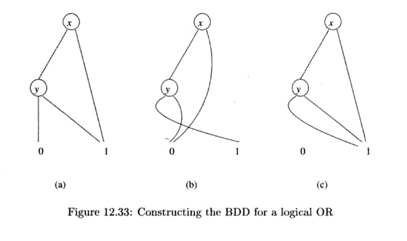
Notice that their logical OR is the function 1 that is always true. To apply Algorithm 12.29 to these two BDD's, we consider the low children of the two roots and the high children of the two roots; let us take up the latter first.

The high child of the root in Fig. 12.33(a) is 1, and in Fig. 12.33(b) it is 0. Since these children are both at the leaf level, we do not have to insert nodes labeled y along each edge, although the result would be the same had we chosen to do so. The basis case for the union of 0 and 1 is to produce a leaf labeled 1 that will become the high child of the new root.

The low children of the roots in Fig.  12.33(a) and (b)  are both labeled y, so we can compute their union BDD recursively.  These two nodes have low children labeled 0 and  1, so the combination of their low children is the leaf labeled 1.  Likewise, their high children are 1  and 0,  so the combination is again the leaf 1.  When we add a new root labeled x, we have the BDD seen in Fig. 12.33(c).

We are not done, since Fig. 12.33(c) can be simplified. The node labeled y has both children the node 1, so we can delete the node y and have the leaf 1 be the low child of the root. Now, both children of the root are the leaf 1, so we can eliminate the root. That is, the simplest BDD for the union is the leaf 1, all by itself. •

5. Using BDD's for Points-to Analysis

Getting context-insensitive points-to analysis to work is already nontrivial. The ordering of the BDD variables can greatly change the size of the representation. Many considerations, as well as trial and error, are needed to come up with an ordering that allows the analysis to complete quickly.

It is even harder to get context-sensitive points-to analysis to execute be-cause of the exponentially many contexts in the program. In particular, if we arbitrarily assign numbers to represent contexts in a call graph, we cannot han-dle even small Java programs. It is important that the contexts be numbered so that the binary encoding of the points-to analysis can be made very com-pact. Two contexts of the same method with similar call paths share a lot of commonalities, so it is desirable to number the n contexts of a method consecu-tively. Similarly, because pairs of caller-callees for the same call site share many similarities, we wish to number the contexts such that the numeric difference between each caller-callee pair of a call site is always a constant.

Even with a clever numbering scheme for the calling contexts, it is still hard to analyze large Java programs efficiently. Active machine learning has been found useful in deriving a variable ordering efficient enough to handle large applications.

6. Exercises for Section 12.7

Exercise 1 2 . 7 . 1 :  Using the encoding of symbols in Example 12.28, develop

a BDD that represents the relation consisting of the tuples  (6, b),  (c, a),  and

(6, a). You may order the boolean variables in whatever way gives you the most succinct BDD.

! Exercise 1 2 . 7 . 2 : As a function of n, how many nodes are there in the most succinct BDD that represents the exclusive-or function on n variables. That is, the function is true if an odd number of the n variables are true and false if an even number are true.

Exercise 1 2 . 7 . 3 : Modify Algorithm 12.29 so it produces the intersection (logical AND) of two BDD's.

Exercise 12 . 7 . 4: Find algorithms to perform the following relational opera-tions on the ordered BDD's that represent them:

a) Project out some of the boolean variables. That is, the function repre-sented should be true for a given truth assignment a if there was any truth assignment for the missing variables that, together with a made the original function true.

b) Join two relations r and s, by combining a tuple from r with one from s whenever these tuples agree on the attributes that r and s have in common. It is really sufficient to consider the case where the relations have only two components, and one from each relation matches; that is, the relations are r(A,B) and s(B, C).

Summary of Chapter 12

Interprocedural Analysis: A data-flow analysis that tracks information across procedure boundaries is said to be interprocedural. Many analyses, such as points-to analysis, can only be done in a meaningful way if they are interprocedural.

• Call Sites: Programs call procedures at certain points referred to as call sites. The procedure called at a site may be obvious, or it may be am-biguous, should the call be indirect through a pointer or a call of a virtual method that has several implementations.

• Call Graphs: A call graph for a program is a bipartite graph with nodes for call sites and nodes for procedures. An edge goes from a call-site node to a procedure node if that procedure may be called at the site.

• Inlining: As long as there is no recursion in a program, we can in principle replace all procedure calls by copies of their code, and use intraprocedural analysis on the resulting program. This analysis is in effect, interproce-dural.

• Flow Sensitivity and Context-Sensitivity: A data-flow analysis that produces facts that depend on location in the program is said to be flowsensitive. If the analysis produces facts that depend on the history of procedure calls is said to be context-sensitive. A data-flow analysis can be either flow- or context-sensitive, both, or neither.

+ Cloning-Based Context-Sensitive Analysis: In principle, once we establish the different contexts in which a procedure can be called, we can imagine that there is a clone of each procedure for each context. In that way, a context-insensitive analysis serves as a context-sensitive analysis.

4- Summary-Based Context-Sensitive Analysis: Another approach to inter-procedural analysis extends the region-based analysis technique that was described for intraprocedural analysis. Each procedure has a transfer function and is treated as a region at each place where that procedure is called.

+ Applications of Interprocedural Analysis: An important application re-quiring interprocedural analysis is the detection of software vulnerabili-ties. These are often characterized by having data read from an untrusted input source by one procedure and used in an exploitable way by another procedure.

•               Datalog: The language Datalog is a simple notation for if-then rules that can be used to describe data-flow analyses at a high level. Collections of Datalog rules, or Datalog programs, can be evaluated using one of several standard algorithms.

Datalog Rules: A Datalog rule consists of a body (antecedent) and head (consequent). The body is one or more atoms, and the head is an atom. Atoms are predicates applied to arguments that are variables or constants.

The atoms of the body are connected by logical AND, and an atom in the body may be negated.

+ IDB and EDB Predicates: EDB predicates in a Datalog program have their true facts given a-priori. In a data-flow analysis, these predicates correspond to the facts that can be obtained from the code being analyzed. IDB predicates are defined by the rules themselves and correspond in a data-flow analysis to the information we are trying to extract from the code being analyzed.

+ Evaluation of Datalog programs: We apply rules by substituting constants for variables that make the body true. Whenever we do so, we infer that the head, with the same substitution for variables, is also true. This operation is repeated, until no more facts can be inferred.

+ Incremental Evaluation of Datalog Programs: An efficiency improvement is obtained by doing incremental evaluation. We perform a series of rounds. In one round, we consider only substitutions of constants for variables that make at least one atom of the body be a fact that was just discovered on the previous round.

+ Java Pointer Analysis: We can model pointer analysis in Java by a frame-work in which there are reference variables that point to heap objects, which may have fields that point to other heap objects. An insensitive pointer analysis can be written as a Datalog program that infers two kinds of facts: a variable can point to a heap object, or a field of a heap object can point to another heap object.

+ Type Information to Improve Pointer Analysis: We can get more precise pointer analysis if we take advantage of the fact that reference variables can only point to heap objects that are of the same type as the variable or a subtype.

• Interprocedural Pointer Analysis: To make the analysis interprocedural, we must add rules that reflect how parameters are passed and return values assigned to variables. These rules are essentially the same as the rules for copying one reference variable to another.

•             Call-Graph Discovery: Since Java has virtual methods, interprocedural analysis requires that we first limit what procedures can be called at a given call site. The principal way to discover limits on what can be called where is to analyze the types of objects and take advantage of the fact that the actual method referred to by a virtual method call must belong to an appropriate class.

Context-Sensitive Analysis: When procedures are recursive, we must con-dense the information contained in call strings into a finite number of contexts. An effective way to do so is to drop from the call string any call site where a procedure calls another procedure (perhaps itself) with which it is mutually recursive. Using this representation, we can modify the rules for intraprocedural pointer analysis so the context is carried along in predicates; this approach simulates cloning-based analysis.

 Binary Decision Diagrams: BDD's are a succinct representation of boolean functions by rooted DAG's. The interior nodes correspond to boolean variables and have two children, low (representing truth value 0) and high (representing 1). There are two leaves labeled 0 and 1. A truth assignment makes the represented function true if and only if the path from the root in which we go to the low child if the variable at a node is 0 and to the high child otherwise, leads to the 1 leaf.

 BDD's and Relations: A BDD can serve as a succinct representation of one of the predicates in a Datalog program. Constants are encoded as truth assignments to a collection of boolean variables, and the function represented by the BDD is true if an only if the boolean variables represent a true fact for that predicate.

 Implementing Data-Flow Analysis by BDD's: Any data-flow analysis that can be expressed as Datalog rules can be implemented by manipulations on the BDD's that represent the predicates involved in those rules. Often, this representation leads to a more efficient implementation of the data-flow analysis than any other known approach.