Context-Sensitive Pointer Analysis

Context-Sensitive Pointer Analysis

1 Contexts and Call Strings

2 Adding Context to Datalog Rules

3 Additional Observations About Sensitivity

4 Exercises for Section 12.6

As discussed in Section 12.1.2, context sensitivity can improve greatly the pre-cision of interprocedural analysis. We talked about two approaches to interpro-cedural analysis, one based on cloning (Section 12.1.4) and one on summaries (Section 12.1.5). Which one should we use?

There are several difficulties in computing the summaries of points-to infor-mation. First, the summaries are large. Each method's summary must include the effect of all the updates that the function and all its callees can make, in terms of the incoming parameters. That is, a method can change the points-to sets of all data reachable through static variables, incoming parameters and all objects created by the method and its callees. While complicated schemes have been proposed, there is no known solution that can scale to large programs. Even if the summaries can be computed in a bottom-up pass, computing the points-to sets for all the exponentially many contexts in a typical top-down pass presents an even greater problem. Such information is necessary for global queries like finding all points in the code that touch a certain object.

In this section, we discuss a cloning-based context-sensitive analysis. A cloning-based analysis simply clones the methods, one for each context of in-terest. We then apply the context-insensitive analysis to the cloned call graph. While this approach seems simple, the devil is in the details of handling the large number of clones. How many contexts are there? Even if we use the idea of collapsing all recursive cycles, as discussed in Section 12.1.3, it is not uncommon to find 1 0 ^{1 4} contexts in a Java application. Representing the results of these many contexts is the challenge.

We separate the discussion of context sensitivity into two parts:

1.          How to handle context sensitivity logically? This part is easy, because we simply apply the context-insensitive algorithm to the cloned call graph.

2.          How to represent the exponentially many contexts? One way is to rep-resent the information as binary decision diagrams (BDD's), a highly-optimized data structure that has been used for many other applications.

This approach to context sensitivity is an excellent example of the impor-tance of abstraction. As we are going to show, we eliminate algorithmic com-plexity by leveraging the years of work that went into the BDD abstraction. We can specify a context-sensitive points-to analysis in just a few lines of Datalog, which in turn takes advantage of many thousands of lines of existing code for BDD manipulation. This approach has several important advantages. First, it makes possible the easy expression of further analyses that use the results of the points-to analysis. After all, the points-to results on their own are not interesting.  Second, it makes it much easier to write the analysis correctly, as it leverages many lines of well-debugged code.

1. Contexts and Call Strings

The context-sensitive points-to analysis described below assumes that a call graph has been already computed. This step helps make possible a compact representation of the many calling contexts. To get the call graph, we first run a context-insensitive points-to analysis that computes the call graph on the fly, as discussed in Section 12.5. We now describe how to create a cloned call graph.

A context is a representation of the call string that forms the history of the active function calls. Another way to look at the context is that it is a summary of the sequence of calls whose activation records are currently on the run-time stack. If there are no recursive functions on the stack, then the call string — the sequence of locations from which the calls on the stack were made — is a complete representation. It is also an acceptable representation, in the sense that there is only a finite number of different contexts, although that number may be exponential in the number of functions in the program.

However, if there are recursive functions in the program, then the number of possible call strings is infinite, and we cannot allow all possible call strings to represent distinct contexts. There are various ways we can limit the number of distinct contexts. For example, we can write a regular expression that describes all possible call strings and convert that regular expression to a deterministic finite automaton, using the methods of Section 3.7. The contexts can then be identified with the states of this automaton.

Here, we shall adopt a simpler scheme that captures the history of nonrecur-sive calls but considers recursive calls to be "too hard to unravel." We begin by finding all the mutually recursive sets of functions in the program. The process is simple and will not be elaborated in detail here. Think of a graph whose nodes are the functions, with an edge from p to q if function p calls function

The strongly connected components (SCC's) of this graph are the sets of mutually recursive functions. As a common special function p that calls itself, but is not in an SCC with any other function is an SCC by itself. The nonrecursive functions are also SCC's by themselves. Call an SCC nontrivial if it either has more than one member (the mutually recursive case), or it has a single, recursive member. The SCC's that are single, nonrecursive functions are trivial SCC's.

Our modification of the rule that any call string is a context is as follows. Given a call string, delete the occurrence of a call site s if

1. s is in a function p.

2. Function q is called at site s (q = p is possible).

3. p and q are in the same strong component (i.e., p and q are mutually recursive, or p = q and p is recursive).

The result is that when a member of a nontrivial SCC S is called, the call site for that call becomes part of the context, but calls within S to other functions in the same SCC are not part of the context. Finally, when a call outside 5 is made, we record that call site as part of the context.

Example 1 2 . 2 6 : In Fig. 12.28 is a sketch of five methods with some call sites and calls among them. An examination of the calls shows that q and r are mutually recursive. However, p, s, and t are not recursive at all. Thus, our contexts will be lists of all the call sites except s3 and s5, where the recursive calls between q and r take place.

Let us consider all the ways we could get from p to t, that is, all the contexts in which calls to t occur:

1.          p could call s at s2, and then s could call t at either s7 or s8. Thus, two possible call strings are (s2, s7) and (s2, s8).

2. p could call q at s 1 . Then, q and r could call each other recursively some number of times. We could break the cycle:

(a) At s4, where t is called directly by q. This choice leads to only one context, ( s 1 , s4).

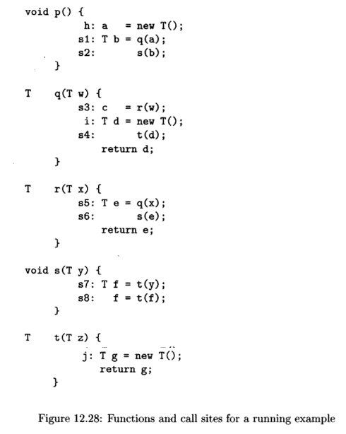
(b) At s6, where r calls s. Here, we can reach t either by the call at s7 or the call at s8. That gives us two more contexts, ( s1 , s6, s7) and

(sl,s6, s8).

There are thus five different contexts in which t can be called. Notice that all these contexts omit the recursive call sites, s3 and s5. For example, the context ( s 1 , s4) actually represents the infinite set of call strings ( s 1 , s3, (s5, s3) ⁿ , s4) for all n > 0. • '

We now describe how we derive the cloned call graph. Each cloned method is identified by the method in the program M and a context C. Edges can be derived by adding the corresponding contexts to each of the edges in the original call graph. Recall that there is an edge in the original call graph linking call site S with method M if the predicate invokes (S, M) is true. To add contexts to identify the methods in the cloned call graph, we can define a corresponding CSinvokes predicate such that CSinvokes(S, C, M, D) is true if the call site S in context C calls the D context of method M.

2. Adding Context to Datalog Rules

To find context-sensitive points-to relations, we can simply apply the same context-insensitive points-to analysis to the cloned call graph. Since a method in the cloned call graph is represented by the original method and its context, we revise all the Datalog rules accordingly. For simplicity, the rules below do not include the type restriction, and the _'s are any new variables.

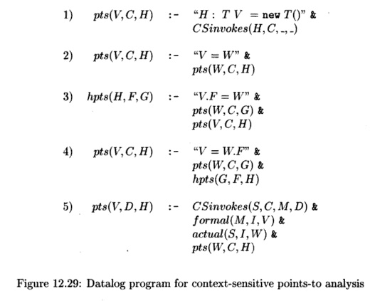
An additional argument, representing the context, must be given to the IDB predicate pts. pts(V, C, H) says that variable V in context C can point to heap object H. All the rules are self-explanatory, perhaps with the exception of Rule 5. Rule 5 says that if the call site 5 in context C calls method M of context D, then the formal parameters in method M of context D can point to the objects pointed to by the corresponding actual parameters in context C.

3. Additional Observations About Sensitivity

What we have described is one formulation of context sensitivity that has been shown to be practical enough to handle many large real-life Java programs, using the tricks described briefly in the next section. Nonetheless, this algorithm cannot yet handle the largest of Java applications.

The heap objects in this formulation are named by their call site, but with-out context sensitivity. That simplification can cause problems. Consider the object-factory idiom where, all objects of the same type are allocated by the same routine. The current scheme would make all objects of that class share the same name. It is relatively simple to handle such cases by essentially inlining the allocation code. In general, it is desirable to increase the context sensitivity in the naming of objects.  While it is easy to add context sensitivity of objects to the Datalog formulation, getting the analysis to scale to large programs is another  matter.

Another important form of sensitivity is object sensitivity. An object-sensitive technique can distinguish between methods invoked on different re-ceiver objects. Consider the scenario of a call site in a calling context where a variable is found to point to two different receiver objects of the same class. Their fields may point to different objects. Without distinguishing between the objects, a copy among fields of the t h i s object reference will create spurious relationships unless we separate the analysis according to the receiver objects. Object sensitivity is more useful than context sensitivity for some analyses.

4. Exercises for Section 12.6

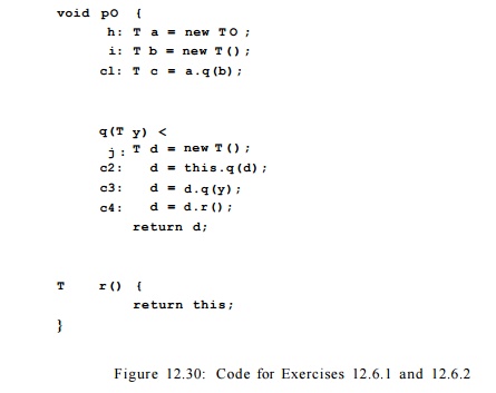
Exercise 12.6.1 : What are all the contexts that would be distinguished if we apply the methods of this section to the code in Fig. 12.30?

Exercise 12.6.2 : Perform a context sensitive analysis of the code in Fig. 12.30.

Exercise 12.6.3: Extend the Datalog rules of this section to incorporate the type and subtype information, following the approach of Section 12.5.