The Simplex Method

The Simplex Method

We have already encountered linear programming (see Section 6.6)—the general problem of optimizing a linear function of several variables subject to a set of linear constraints:

We mentioned there that many important practical problems can be modeled as instances of linear programming. Two researchers, L. V. Kantorovich of the former Soviet Union and the Dutch-American T. C. Koopmans, were even awarded the Nobel Prize in 1975 for their contributions to linear programming theory and its applications to economics. Apparently because there is no Nobel Prize in mathematics, the Royal Swedish Academy of Sciences failed to honor the U.S. mathematician G. B. Dantzig, who is universally recognized as the father of linear  programming in its modern form and the inventor of the simplex method, the classic algorithm for solving such problems.

Geometric Interpretation of Linear Programming

Before we introduce a general method for solving linear programming problems, let us consider a small example, which will help us to see the fundamental prop-erties of such problems.

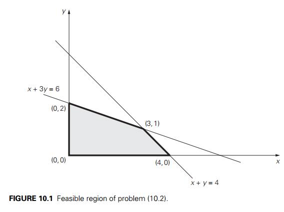
EXAMPLE 1 Consider the following linear programming problem in two variables:

By definition, a feasible solution to this problem is any point (x, y) that satisfies all the constraints of the problem; the problem’s feasible region is the set of all its feasible points. It is instructive to sketch the feasible region in the Cartesian plane. Recall that any equation ax + by = c, where coefficients a and b are not both equal to zero, defines a straight line. Such a line divides the plane into two half-planes: for all the points in one of them, ax + by < c, while for all the points in the other, ax + by > c. (It is easy to determine which of the two half-planes is which: take any point (x₀, y₀) not on the line ax + by = c and check which of the two inequalities hold, ax₀ + by₀ > c or ax₀ + by₀ < c.) In particular, the set of points defined by inequality x + y ≤ 4 comprises the points on and below the line x + y = 4, and the set of points defined by inequality x + 3y ≤ 6 comprises the points on and below the line x + 3y = 6. Since the points of the feasible region must satisfy all the constraints of the problem, the feasible region is obtained by the intersection of these two half-planes and the first quadrant of the Cartesian plane defined by the nonnegativity constraints x ≥ 0, y ≥ 0 (see Figure 10.1). Thus, the feasible region for problem (10.2) is the convex polygon with the vertices (0, 0), (4, 0), (0, 2), and (3, 1). (The last point, which is the point of intersection of the lines x + y = 4 and x + 3y = 6, is obtained by solving the system of these two linear equations.) Our task is to find an optimal solution, a point in the feasible region with the largest value of the objective function z = 3x + 5y.

Are there feasible solutions for which the value of the objective function equals, say, 20? The points (x, y) for which the objective function z = 3x + 5y is equal to 20 form the line 3x + 5y = 20. Since this line does not have common points

with the feasible region—see Figure 10.2—the answer to the posed question is no. On the other hand, there are infinitely many feasible points for which the objective function is equal to, say, 10: they are the intersection points of the line 3x + 5y = 10 with the feasible region. Note that the lines 3x + 5y = 20 and 3x + 5y = 10 have the same slope, as would any line defined by equation 3x + 5y = z where z is some constant. Such lines are called level lines of the objective function. Thus, our problem can be restated as finding the largest value of the parameter z for which the level line 3x + 5y = z has a common point with the feasible region.

We can find this line either by shifting, say, the line 3x + 5y = 20 south-west (without changing its slope!) toward the feasible region until it hits the region for the first time or by shifting, say, the line 3x + 5y = 10 north-east until it hits the feasible region for the last time. Either way, it will happen at the point (3, 1) with the corresponding z value 3 ^. 3 + 5 ^. 1 = 14. This means that the optimal solution to the linear programming problem in question is x = 3, y = 1, with the maximal value of the objective function equal to 14.

Note that if we had to maximize z = 3x + 3y as the objective function in problem (10.2), the level line 3x + 3y = z for the largest value of z would coincide with the boundary line segment that has the same slope as the level lines (draw this line in Figure 10.2). Consequently, all the points of the line segment between vertices (3, 1) and (4, 0), including the vertices themselves, would be optimal solutions, yielding, of course, the same maximal value of the objective function.

Does every linear programming problem have an optimal solution that can be found at a vertex of its feasible region? Without appropriate qualifications, the answer to this question is no. To begin with, the feasible region of a linear programming problem can be empty. For example, if the constraints include two contradictory requirements, such as x + y ≤ 1 and x + y ≥ 2, there can be no points in the problem’s feasible region. Linear programming problems with the empty feasible region are called infeasible. Obviously, infeasible problems do not have optimal solutions.

Another complication may arise if the problem’s feasible region is unbounded, as the following example demonstrates.

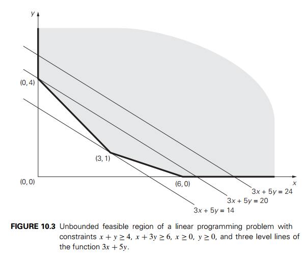
EXAMPLE 2 If we reverse the inequalities in problem (10.2) to x + y ≥ 4 and x + 3y ≥ 6, the feasible region of the new problem will become unbounded (see Figure 10.3). If the feasible region of a linear programming problem is unbounded, its objective function may or may not attain a finite optimal value on it. For example, the problem of maximizing z = 3x + 5y subject to the constraints x + y ≥ 4, x + 3y ≥ 6, x ≥ 0, y ≥ 0 has no optimal solution, because there are points in the feasible region making 3x + 5y as large as we wish. Such problems are called unbounded. On the other hand, the problem of minimizing z = 3x + 5y subject to the same constraints has an optimal solution (which?).

Fortunately, the most important features of the examples we considered above hold for problems with more than two variables. In particular, a feasible region of a typical linear programming problem is in many ways similar to convex polygons in the two-dimensional Cartesian plane. Specifically, it always has a finite number of vertices, which mathematicians prefer to call extreme points (see Section 3.3). Furthermore, an optimal solution to a linear programming problem can be found at one of the extreme points of its feasible region. We reiterate these properties in the following theorem.

THEOREM (Extreme Point Theorem) Any linear programming problem with a nonempty bounded feasible region has an optimal solution; moreover, an op-timal solution can always be found at an extreme point of the problem’s feasible region.²

This theorem implies that to solve a linear programming problem, at least in the case of a bounded feasible region, we can ignore all but a finite number of points in its feasible region. In principle, we can solve such a problem by computing the value of the objective function at each extreme point and selecting the one with the best value. There are two major obstacles to implementing this plan, however. The first lies in the need for a mechanism for generating the extreme points of the feasible region. As we are going to see below, a rather straightforward algebraic procedure for this task has been discovered. The second obstacle lies in the number of extreme points a typical feasible region has. Here, the news is bad: the number of extreme points is known to grow exponentially with the size of the problem. This makes the exhaustive inspection of extreme points unrealistic for most linear programming problems of nontrivial sizes.

Fortunately, it turns out that there exists an algorithm that typically inspects only a small fraction of the extreme points of the feasible region before reaching an optimal one. This famous algorithm is called the simplex method. The idea of this algorithm can be described in geometric terms as follows. Start by identifying an extreme point of the feasible region. Then check whether one can get an improved value of the objective function by going to an adjacent extreme point. If it is not the case, the current point is optimal—stop; if it is the case, proceed to an adjacent extreme point with an improved value of the objective function. After a finite number of steps, the algorithm will either reach an extreme point where an optimal solution occurs or determine that no optimal solution exists.

An Outline of the Simplex Method

Our task now is to “translate” the geometric description of the simplex method into the more algorithmically precise language of algebra. To begin with, before we can apply the simplex method to a linear programming problem, it has to be represented in a special form called the standard form. The standard form has the following requirements:

It must be a maximization problem.

All the constraints (except the nonnegativity constraints) must be in the form of linear equations with nonnegative right-hand sides.

All the variables must be required to be nonnegative.

Thus, the general linear programming problem in standard form with m constraints and n unknowns (n ≥ m) is

Any linear programming problem can be transformed into an equivalent problem in standard form. If an objective function needs to be minimized, it can be replaced by the equivalent problem of maximizing the same objective function with all its coefficients c_j replaced by −c_j , j = 1, 2, . . . , n (see Section 6.6 for a more general discussion of such transformations). If a constraint is given as an inequality, it can be replaced by an equivalent equation by adding a slack variable representing the difference between the two sides of the original inequality. For example, the two inequalities of problem (10.2) can be transformed, respectively, into the following equations:

x + y + u = 4 where u ≥ 0  and x + 3y + v = 6 where v ≥ 0.

Finally, in most linear programming problems, the variables are required to be nonnegative to begin with because they represent some physical quantities. If this is not the case in an initial statement of a problem, an unconstrained variable

x_j can be replaced by the difference between two new nonnegative variables: x_j = x'_j − x''_j , x'_j ≥ 0, x''_j ≥ 0.

Thus, problem (10.2) in standard form is the following linear programming problem in four variables:

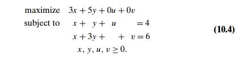
It is easy to see that if we find an optimal solution (x^∗, y^∗, u^∗, v^∗) to problem (10.4), we can obtain an optimal solution to problem (10.2) by simply ignoring its last two coordinates.

The principal advantage of the standard form lies in the simple mechanism it provides for identifying extreme points of the feasible region. To do this for problem (10.4), for example, we need to set two of the four variables in the con-straint equations to zero to get a system of two linear equations in two unknowns and solve this system. For the general case of a problem with m equations in n unknowns (n ≥ m), n − m variables need to be set to zero to get a system of m equations in m unknowns. If the system obtained has a unique solution—as any nondegenerate system of linear equations with the number of equations equal to the number of unknowns does—we have a basic solution; its coordinates set to zero before solving the system are called nonbasic, and its coordinates obtained by solving the system are called basic. (This terminology comes from linear algebra.

Specifically, we can rewrite the system of constraint equations of (10.4) as

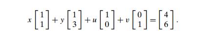
A basis in the two-dimensional vector space is composed of any two vectors that are not proportional to each other; once a basis is chosen, any vector can be uniquely expressed as a sum of multiples of the basis vectors. Basic and nonba-sic variables indicate which of the given vectors are, respectively, included and excluded in a particular basis choice.)

If all the coordinates of a basic solution are nonnegative, the basic solution is called a basic feasible solution. For example, if we set to zero variables x and y and solve the resulting system for u and v, we obtain the basic feasible solution (0, 0, 4, 6); if we set to zero variables x and u and solve the resulting system for y and v, we obtain the basic solution (0, 4, 0, −6), which is not feasible. The impor-tance of basic feasible solutions lies in the one-to-one correspondence between them and the extreme points of the feasible region. For example, (0, 0, 4, 6) is an extreme point of the feasible region of problem (10.4) (with the point (0, 0) in Fig-ure 10.1 being its projection on the x, y plane). Incidentally, (0, 0, 4, 6) is a natural starting point for the simplex method’s application to this problem.

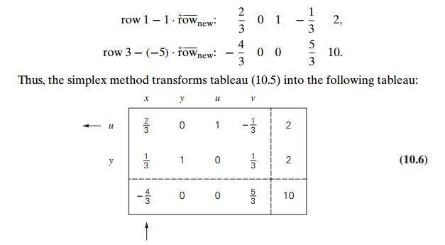
As mentioned above, the simplex method progresses through a series of adjacent extreme points (basic feasible solutions) with increasing values of the objective function. Each such point can be represented by a simplex tableau, a table storing the information about the basic feasible solution corresponding to the extreme point. For example, the simplex tableau for (0, 0, 4, 6) of problem (10.4) is presented below:

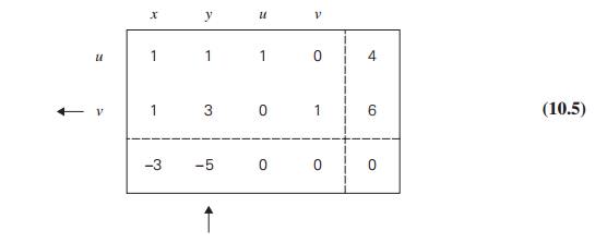
In general, a simplex tableau for a linear programming problem in standard form with n unknowns and m linear equality constraints (n ≥ m) has m + 1 rows and n + 1 columns. Each of the first m rows of the table contains the coefficients of a corresponding constraint equation, with the last column’s entry containing the equation’s right-hand side. The columns, except the last one, are labeled by the names of the variables. The rows are labeled by the basic variables of the basic feasible solution the tableau represents; the values of the basic variables of this solution are in the last column. Also note that the columns labeled by the basic variables form the m × m identity matrix.

The last row of a simplex tableau is called the objective row. It is initialized by the coefficients of the objective function with their signs reversed (in the first n columns) and the value of the objective function at the initial point (in the last column). On subsequent iterations, the objective row is transformed the same way as all the other rows. The objective row is used by the simplex method to check whether the current tableau represents an optimal solution: it does if all the entries in the objective row—except, possibly, the one in the last column—are nonnegative. If this is not the case, any of the negative entries indicates a nonbasic variable that can become basic in the next tableau.

For example, according to this criterion, the basic feasible solution (0, 0, 4, 6) represented by tableau (10.5) is not optimal. The negative value in the x-column signals the fact that we can increase the value of the objective function z = 3x + 5y + 0u + 0v by increasing the value of the x-coordinate in the current basic feasible solution (0, 0, 4, 6). Indeed, since the coefficient for x in the objective function is positive, the larger the x value, the larger the value of this function. Of course, we will need to “compensate” an increase in x by adjusting the values of the basic variables u and v so that the new point is still feasible. For this to be the case, both conditions

x + u = 4 where u ≥ 0 x + v = 6 where v ≥ 0

must be satisfied, which means that

x ≤ min{4, 6} = 4.

Note that if we increase the value of x from 0 to 4, the largest amount possible, we will find ourselves at the point (4, 0, 0, 2), an adjacent to (0, 0, 4, 6) extreme point of the feasible region, with z = 12.

Similarly, the negative value in the y-column of the objective row signals the fact that we can also increase the value of the objective function by increasing the value of the y-coordinate in the initial basic feasible solution (0, 0, 4, 6). This requires

y + u = 4 where u ≥ 0 3y + v = 6 where v ≥ 0,

which means that

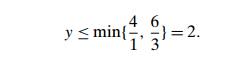
If we increase the value of y from 0 to 2, the largest amount possible, we will find ourselves at the point (0, 2, 2, 0), another adjacent to (0, 0, 4, 6) extreme point, with z = 10.

If there are several negative entries in the objective row, a commonly used rule is to select the most negative one, i.e., the negative number with the largest absolute value. This rule is motivated by the observation that such a choice yields the largest increase in the objective function’s value per unit of change in a vari-able’s value. (In our example, an increase in the x-value from 0 to 1 at (0, 0, 4, 6) changes the value of z = 3x + 5y + 0u + 0v from 0 to 3, while an increase in the y-value from 0 to 1 at (0, 0, 4, 6) changes z from 0 to 5.) Note, however, that the feasibility constraints impose different limits on how much each of the variables may increase. In our example, in particular, the choice of the y-variable over the x-variable leads to a smaller increase in the value of the objective function. Still, we will employ this commonly used rule and select variable y as we continue with our example. A new basic variable is called the entering variable, while its column is referred to as the pivot column; we mark the pivot column by ↑ .

Now we will explain how to choose a departing variable, i.e., a basic variable to become nonbasic in the next tableau. (The total number of basic variables in any basic solution must be equal to m, the number of the equality constraints.) As we saw above, to get to an adjacent extreme point with a larger value of the objective function, we need to increase the entering variable by the largest amount possible to make one of the old basic variables zero while preserving the nonnegativity of all the others. We can translate this observation into the following rule for choosing a departing variable in a simplex tableau: for each positive entry in the pivot column, compute the θ -ratio by dividing the row’s last entry by the entry in the pivot column. For the example of tableau (10.5), these θ -ratios are

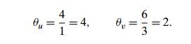
The row with the smallest θ -ratio determines the departing variable, i.e., the variable to become nonbasic. Ties may be broken arbitrarily. For our example, it is variable v. We mark the row of the departing variable, called the pivot row, by ←

and denote it row. Note that if there are no positive entries in the pivot column, no θ -ratio can be computed, which indicates that the problem is unbounded and the algorithm stops.

Finally, the following steps need to be taken to transform a current tableau into the next one. (This transformation, called pivoting, is similar to the princi-pal step of the Gauss-Jordan elimination algorithm for solving systems of linear equations—see Problem 8 in Exercises 6.2.) First, divide all the entries of the pivot

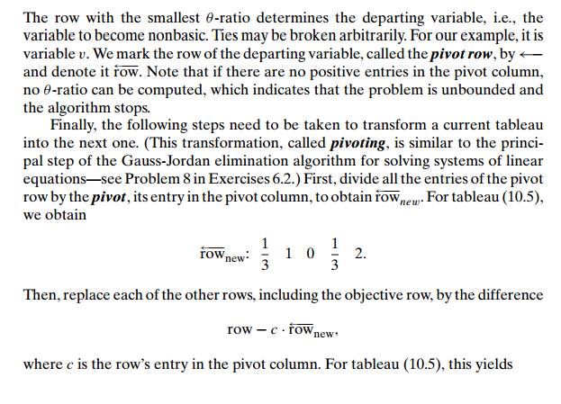
Tableau (10.6) represents the basic feasible solution (0, 2, 2, 0) with an increased value of the objective function, which is equal to 10. It is not optimal, however (why?).

The next iteration—do it yourself as a good exercise!—yields tableau (10.7):

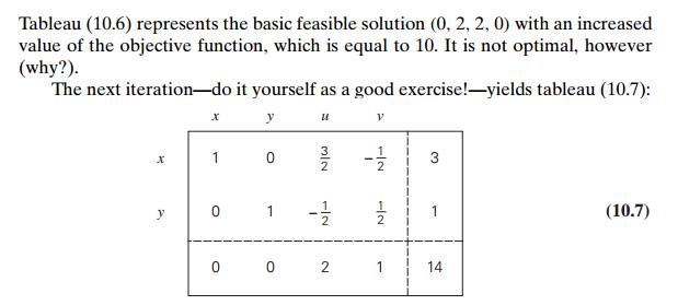
This tableau represents the basic feasible solution (3, 1, 0, 0). It is optimal because all the entries in the objective row of tableau (10.7) are nonnegative. The maximal value of the objective function is equal to 14, the last entry in the objective row.

Let us summarize the steps of the simplex method.

Summary of the simplex method

Step 0 Initialization Present a given linear programming problem in stan-dard form and set up an initial tableau with nonnegative entries in the rightmost column and m other columns composing the m × m identity matrix. (Entries in the objective row are to be disregarded in verifying these requirements.) These m columns define the basic variables of the initial basic feasible solution, used as the labels of the tableau’s rows.

Step 1 Optimality test If all the entries in the objective row (except, possibly, the one in the rightmost column, which represents the value of the objective function) are nonnegative—stop: the tableau represents an optimal solution whose basic variables’ values are in the rightmost column and the remaining, nonbasic variables’ values are zeros.

Step 2 Finding the entering variable Select a negative entry from among the first n elements of the objective row. (A commonly used rule is to select the negative entry with the largest absolute value, with ties broken arbitrarily.) Mark its column to indicate the entering variable and the pivot column.

Step 3 Finding the departing variable For each positive entry in the pivot column, calculate the θ -ratio by dividing that row’s entry in the right-most column by its entry in the pivot column. (If all the entries in the pivot column are negative or zero, the problem is unbounded—stop.) Find the row with the smallest θ -ratio (ties may be broken arbitrarily), and mark this row to indicate the departing variable and the pivot row.

Step 4 Forming the next tableau Divide all the entries in the pivot row by its entry in the pivot column. Subtract from each of the other rows, including the objective row, the new pivot row multiplied by the entry in the pivot column of the row in question. (This will make all the entries in the pivot column 0’s except for 1 in the pivot row.) Replace the label of the pivot row by the variable’s name of the pivot column and go back to Step 1.

Further Notes on the Simplex Method

Formal proofs of validity of the simplex method steps can be found in books devoted to a detailed discussion of linear programming (e.g., [Dan63]). A few important remarks about the method still need to be made, however. Generally speaking, an iteration of the simplex method leads to an extreme point of the prob-lem’s feasible region with a greater value of the objective function. In degenerate cases, which arise when one or more basic variables are equal to zero, the simplex method can only guarantee that the value of the objective function at the new extreme point is greater than or equal to its value at the previous point. In turn, this opens the door to the possibility not only that the objective function’s values “stall” for several iterations in a row but that the algorithm might cycle back to a previously considered point and hence never terminate. The latter phenomenon is called cycling. Although it rarely if ever happens in practice, specific examples of problems where cycling does occur have been constructed. A simple modifica-tion of Steps 2 and 3 of the simplex method, called Bland’s rule, eliminates even the theoretical possibility of cycling. Assuming that the variables are denoted by a subscripted letter (e.g., x₁, x₂, . . . , x_n), this rule can be stated as follows:

Step 2 modified Among the columns with a negative entry in the objective row, select the column with the smallest subscript.

Step 3 modified Resolve a tie among the smallest θ -ratios by selecting the row labeled by the basic variable with the smallest subscript.

Another caveat deals with the assumptions made in Step 0. They are automat-ically satisfied if a problem is given in the form where all the constraints imposed on nonnegative variables are inequalities a_i1x₁ + ^{. . .} + a_inx_n ≤ b_i with b_i ≥ 0 for i = 1, 2, . . . , m. Indeed, by adding a nonnegative slack variable x_n+i into the ith constraint, we obtain the equality a_i1x₁ + ^{. . .} + a_inx_n + x_n+i = b_i, and all the re-quirements imposed on an initial tableau of the simplex method are satisfied for

the obvious basic feasible solution x₁ = ^{. . .} = x_n = 0, x_n+1 = ^{. . .} = x_n+m = 1. But if a problem is not given in such a form, finding an initial basic feasible solution

may present a nontrivial obstacle. Moreover, for problems with an empty feasible region, no initial basic feasible solution exists, and we need an algorithmic way to identify such problems. One of the ways to address these issues is to use an exten-sion to the classic simplex method called the two-phase simplex method (see, e.g., [Kol95]). In a nutshell, this method adds a set of artificial variables to the equality constraints of a given problem so that the new problem has an obvious basic fea-sible solution. It then solves the linear programming problem of minimizing the sum of the artificial variables by the simplex method. The optimal solution to this problem either yields an initial tableau for the original problem or indicates that the feasible region of the original problem is empty.

How efficient is the simplex method? Since the algorithm progresses through a sequence of adjacent points of a feasible region, one should probably expect bad news because the number of extreme points is known to grow exponentially with the problem size. Indeed, the worst-case efficiency of the simplex method has been shown to be exponential as well. Fortunately, more than half a century of practical experience with the algorithm has shown that the number of iterations in a typical application ranges between m and 3m, with the number of operations per iteration proportional to mn, where m and n are the numbers of equality constraints and variables, respectively.

Since its discovery in 1947, the simplex method has been a subject of intensive study by many researchers. Some of them have worked on improvements to the original algorithm and details of its efficient implementation. As a result of these efforts, programs implementing the simplex method have been polished to the point that very large problems with hundreds of thousands of constraints and variables can be solved in a routine manner. In fact, such programs have evolved into sophisticated software packages. These packages enable the user to enter a problem’s constraints and obtain a solution in a user-friendly form. They also provide tools for investigating important properties of the solution, such as its sensitivity to changes in the input data. Such investigations are very important for many applications, including those in economics. At the other end of the spectrum, linear programming problems of a moderate size can nowadays be solved on a desktop using a standard spreadsheet facility or by taking advantage of specialized software available on the Internet.

Researchers have also tried to find algorithms for solving linear programming problems with polynomial-time efficiency in the worst case. An important mile-stone in the history of such algorithms was the proof by L. G. Khachian [Kha79] showing that the ellipsoid method can solve any linear programming problem in polynomial time. Although the ellipsoid method was much slower than the simplex method in practice, its better worst-case efficiency encouraged a search for alterna-tives to the simplex method. In 1984, Narendra Karmarkar published an algorithm that not only had a polynomial worst-case efficiency but also was competitive with the simplex method in empirical tests as well. Although we are not going to discuss Karmarkar’s algorithm [Kar84] here, it is worth pointing out that it is also based on the iterative-improvement idea. However, Karmarkar’s algorithm generates a sequence of feasible solutions that lie within the feasible region rather than going through a sequence of adjacent extreme points as the simplex method does. Such algorithms are called interior-point methods (see, e.g., [Arb93]).

Exercises 10.1

            Consider the following version of the post office location problem (Problem 3 in Exercises 3.3): Given n integers x₁, x₂, . . . , x_n representing coordinates of n villages located along a straight road, find a location for a post office that minimizes the average distance between the villages. The post office may be, but is not required to be, located at one of the villages. Devise an iterative-improvement algorithm for this problem. Is this an efficient way to solve this problem?

Solve the following linear programming problems geometrically.

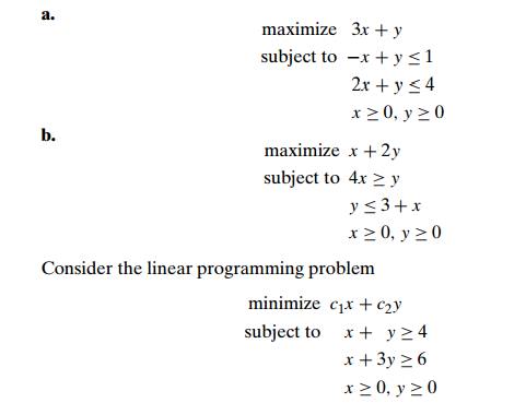
where c₁ and c₂ are some real numbers not both equal to zero.

Give an example of the coefficient values c₁ and c₂ for which the problem has a unique optimal solution.

            Give an example of the coefficient values c₁ and c₂ for which the problem has infinitely many optimal solutions.

            Give an example of the coefficient values c₁ and c₂ for which the problem does not have an optimal solution.

            Would the solution to problem (10.2) be different if its inequality constraints were strict, i.e., x + y < 4 and x + 3y < 6, respectively?

            Trace the simplex method on

            the problem of Exercise 2a.

            the problem of Exercise 2b.

            Trace the simplex method on the problem of Example 1 in Section 6.6

            by hand.

            by using one of the implementations available on the Internet.

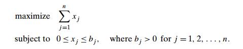
            Determine how many iterations the simplex method needs to solve the problem

            Can we apply the simplex method to solve the knapsack problem (see Exam-ple 2 in Section 6.6)? If you answer yes, indicate whether it is a good algorithm for the problem in question; if you answer no, explain why not.

            Prove that no linear programming problem can have exactly k ≥ 1 optimal solutions unless k = 1.

            If a linear programming problem

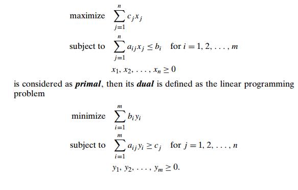
            Express the primal and dual problems in matrix notations.

            Find the dual of the linear programming problem

maximize x₁ + 4x₂ − x₃ subject to x₁ + x₂ + x₃ ≤ 6

x₁ − x₂ − 2x₃ ≤ 2 x₁, x₂, x₃ ≥ 0.

            Solve the primal and dual problems and compare the optimal values of their objective functions.