Chapter: Introduction to the Design and Analysis of Algorithms : Iterative Improvement
The Iterative Maximum-Flow Problem
The Maximum-Flow Problem
In this section, we consider
the important problem of maximizing the flow of a ma-terial through a
transportation network (pipeline system, communication system, electrical
distribution system, and so on). We will assume that the transportation network
in question can be represented by a connected weighted digraph with n vertices numbered from 1 to n and a set of edges E, with the following properties:
It contains exactly one
vertex with no entering edges; this vertex is called the source and assumed to be
numbered 1.
It contains exactly one vertex
with no leaving edges; this vertex is called the sink and assumed to be
numbered n.
The weight uij of each directed edge (i, j ) is a positive integer, called the edge capacity.
(This number represents the upper bound on the amount of the material that can
be sent from i to j through a link represented by this edge.)
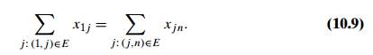
A digraph satisfying these
properties is called a flow network or simply a network.3 A small instance of a network
is given in Figure 10.4.
It is assumed that the source
and the sink are the only source and destination of the material, respectively;
all the other vertices can serve only as points where a flow can be redirected
without consuming or adding any amount of the material. In other words, the
total amount of the material entering an intermediate vertex must be equal to
the total amount of the material leaving the vertex. This con-dition is called
the flow-conservation
requirement. If we denote the amount sent through edge (i, j ) by xij , then for any intermediate
vertex i, the flow-conservation
requirement can be expressed by the following equality constraint:
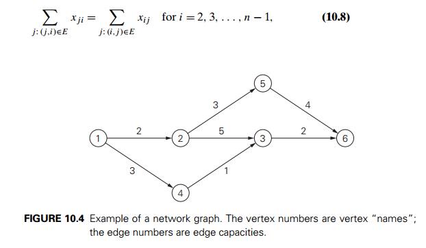
where the sums in the left-
and right-hand sides express the total inflow and outflow entering and leaving
vertex i, respectively.
Since no amount of the
material can change by going through intermediate vertices of the network, it
stands to reason that the total amount of the material leaving the source must
end up at the sink. (This observation can also be derived formally from
equalities (10.8), a task you will be asked to do in the exercises.) Thus, we
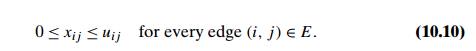
have the following equality:
This quantity, the total
outflow from the source—or, equivalently, the total inflow into the sink—is
called the value of the flow. We denote it by v. It is this quantity that we will want to
maximize over all possible flows in a network.
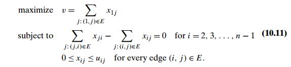
Thus, a (feasible) flow
is an assignment of real numbers xij to edges (i, j ) of a given network that satisfy
flow-conservation constraints (10.8) and the capacity constraints
The maximum-flow problem can
be stated formally as the following optimization problem:
We can solve linear
programming problem (10.11) by the simplex method or by another algorithm for
general linear programming problems (see Section 10.1). However, the special
structure of problem (10.11) can be exploited to design faster algorithms. In particular,
it is quite natural to employ the iterative-improvement idea as follows. We can
always start with the zero flow (i.e., set xij = 0 for every edge (i, j ) in the network). Then, on each iteration, we
can try to find a path from source to sink along which some additional flow can
be sent. Such a path is called flow augmenting. If a
flow-augmenting path is found, we adjust the flow along the edges of this path
to get a flow of an increased value and try to find an augmenting path for the
new flow. If no flow-augmenting path can be found, we conclude that the current
flow is optimal. This general template for solving the maximum-flow problem is
called the augmenting-path method, also known as the Ford-Fulkerson method
after L. R. Ford, Jr., and D. R. Fulkerson, who discovered it (see [For57]).
An actual implementation of
the augmenting path idea is, however, not quite straightforward. To see this,
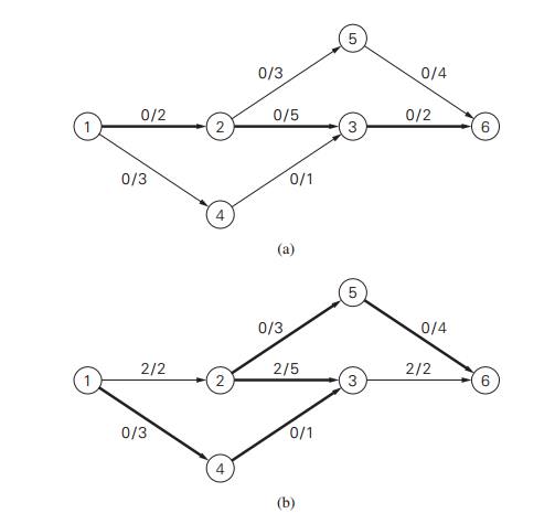
let us consider the network in Figure 10.4. We start with the zero flow shown
in Figure 10.5a. (In that figure, the zero amounts sent through each edge are
separated from the edge capacities by the slashes; we will use this notation in
the other examples as well.) It is natural to search for a flow-augmenting path
from source to sink by following directed edges (i, j ) for which the current flow xij is less than the edge capacity uij . Among several possibilities, let us assume
that we identify the augmenting path 1→2→3→6 first. We can increase the flow along this
path by a maximum of 2 units, which is the smallest unused capacity of its
edges. The new flow is shown in Figure 10.5b. This is as far as our
simpleminded idea about flow-augmenting paths will be able to take us.
Unfortunately, the flow shown in Figure 10.5b is not optimal: its value can
still be increased along the path 1→4→3←2→5→6 by increasing the flow by 1 on edges (1, 4), (4, 3), (2, 5), and (5, 6) and decreasing
it by 1 on edge (2, 3). The flow obtained as the
result of this augmentation is shown in Figure 10.5c. It is indeed maximal.
(Can you tell why?)
Thus, to find a
flow-augmenting path for a flow x, we need to consider paths
from source to sink in the underlying undirected
graph in which any two consec-utive vertices i, j are either
connected by a directed edge from i to j with some positive unused
capacity rij = uij − xij (so that we can increase the flow through that
edge by up to rij units), or
connected by a directed edge from j to i with some positive flow xj i (so that we can decrease the flow through that
edge by up to xj i units).
Edges of the first kind are
called forward edges because their tail is listed before their head in
the vertex list 1 → . . . i → j . . . → n defining the path; edges of
the second kind are called backward edges because their tail is
listed after their head in the path list 1 → . . . i ← j . . . → n. To illustrate, for the path
1→4→3←2→5→6 of the last example, (1, 4), (4, 3), (2, 5), and (5, 6) are the forward edges, and (3, 2) is the backward edge.
For a given flow-augmenting
path, let r be the minimum of all the
unused capacities rij of its forward edges and all the flows xj i of its backward edges. It is easy to see that
if we increase the current flow by r on each forward edge and
decrease it by this amount on each backward edge, we will obtain a feasible
flow whose value is r units greater than the value of its
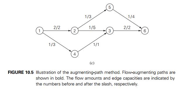
predecessor. Indeed, let i be an intermediate vertex on
a flow-augmenting path. There are four possible combinations of forward and backward edges
incident to vertex i:
For each of them, the
flow-conservation requirement for vertex i will still hold after the flow adjustments
indicated above the edge arrows. Further, since r is the minimum among all the positive unused
capacities on the forward edges and all the positive flows on the backward
edges of the flow-augmenting path, the new flow will satisfy the capacity
constraints as well. Finally, adding r to the flow on the first edge of the
augmenting path will increase the value of the flow by r.
Under the assumption that all
the edge capacities are integers, r will be a positive integer
too. Hence, the flow value increases at least by 1 on each iteration of the
augmenting-path method. Since the value of a maximum flow is bounded above
(e.g., by the sum of the capacities of the source edges), the augmenting-path
method has to stop after a finite number of iterations.4 Surprisingly, the final flow
always turns out to be maximal, irrespective of a sequence of augmenting paths.
This remarkable result stems from the proof of the Max-Flow Min-Cut Theorem
(see, e.g., [For62]), which we replicate later in this section.
The augmenting-path method—as
described above in its general form—does not indicate a specific way for
generating flow-augmenting paths. A bad sequence of such paths may, however,
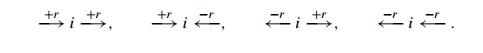
have a dramatic impact on the method’s efficiency. Consider, for example, the
network in Figure 10.6a, in which U stands for some large
positive integer. If we augment the zero flow along the path 1→2→3→4, we shall obtain the flow of value 1 shown in
Figure 10.6b. Augmenting that flow along the path 1→3←2→4 will increase the flow value to 2 (Figure
10.6c). If we continue selecting this pair of flow-augmenting paths, we will
need a total of 2U iterations to reach the
maximum flow of value 2U (Figure 10.6d). Of course,
we can obtain the maximum flow in just two iterations by augmenting the initial
zero flow along the path 1→2→4 followed by augmenting the new flow along the
path 1→3→4. The dramatic difference
between 2U and 2 iterations makes the
point.
Fortunately, there are
several ways to generate flow-augmenting paths ef-ficiently and avoid the
degradation in performance illustrated by the previous example. The simplest of
them uses breadth-first search to generate augment-ing paths with the least
number of edges (see Section 3.5). This version of the augmenting-path method,
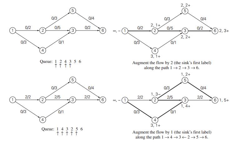
called shortest-augmenting-path or first-labeled-first-scanned
algorithm, was suggested by J. Edmonds and R. M. Karp [Edm72]. The labeling
refers to marking a new (unlabeled) vertex with two labels. The first label
indicates the amount of additional flow that can be brought from the source to
the vertex being labeled. The second label is the name of the vertex from which
the vertex being labeled was reached. (It can be left undefined for the
source.) It is also convenient to add the + or − sign to the second label to indicate whether
the vertex was reached via a forward or backward edge, respectively. The source
can be always labeled with ∞, −. For the other vertices, the labels are
computed as follows.
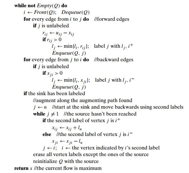
If unlabeled vertex j is connected to the front vertex i of the traversal queue by a directed edge from
i to j with positive unused capacity rij = uij − xij , then
vertex j is labeled with lj ,
i+, where lj = min{li, rij }.
If unlabeled vertex j is connected to the front vertex i of the traversal queue by a directed edge from
j to i with positive flow xj i, then vertex j is labeled with
lj , i−, where lj = min{li, xj i}.
If this labeling-enhanced
traversal ends up labeling the sink, the current flow can be augmented by the
amount indicated by the sink’s first label. The augmentation is performed along
the augmenting path traced by following the vertex second labels from sink to
source: the current flow quantities are increased on the forward edges and
decreased on the backward edges of this path. If, on the other hand, the sink
remains unlabeled after the traversal queue becomes empty, the algorithm
returns the current flow as maximum and stops.
ALGORITHM ShortestAugmentingPath(G)
//Implements the
shortest-augmenting-path algorithm //Input: A network with single source 1,
single sink n, and // positive integer
capacities uij on its edges (i, j ) //Output: A maximum flow x
assign xij = 0 to every edge (i, j ) in the network
label the source with ∞, − and add the source to the empty queue Q
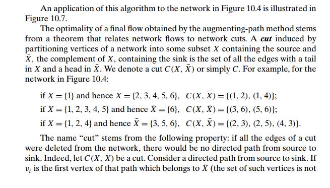

capacities of the edges that
compose the cut. For the three examples of cuts given above, the capacities are
equal to 5, 6, and 9, respectively. Since the number of different cuts in a
network is nonempty and finite (why?), there always exists a minimum
cut, i.e., a cut with the smallest capacity. (What is a minimum cut in
the network of Figure 10.4?) The following theorem establishes an important
relationship between the notions of maximum flow and minimum cut.
THEOREM
(Max-Flow Min-Cut Theorem) The value of a maximum flow
in a network is equal to the capacity of its minimum
cut.
Thus, the value of any
feasible flow in a network cannot exceed the capacity of any cut in that
network.
Let v∗ be the value of a final flow x∗ obtained by the augmenting-path method. If we
now find a cut whose capacity is equal to v∗, we will
have to conclude, in view of inequality (10.13), that (i) the value v∗ of the final flow is maximal among all
feasible flows, (ii) the cut’s capacity is minimal among all cuts in the
network, and
the maximum-flow value is equal to the minimum-cut capacity.
To find
such a cut, consider the set of vertices X∗ that
can be reached from the
source by following an
undirected path composed of forward edges with positive unused capacities (with
respect to the final flow x∗) and backward edges with positive flows on
them. This set contains the source but does not contain the sink: if it did, we
would have an augmenting path for the flow x∗, which would
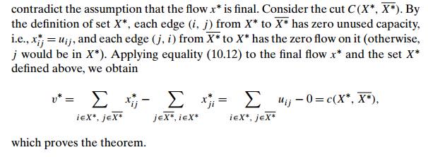
The proof outlined above
accomplishes more than proving the equality of the maximum-flow value and the
minimum-cut capacity. It also implies that when the augmenting-path method
terminates, it yields both a maximum flow and a mini-mum cut. If labeling of
the kind utilized in the shortest-augmenting-path algorithm is used, a minimum
cut is formed by the edges from the labeled to unlabeled ver-tices on the last
iteration of the method. Finally, the proof implies that all such edges must be
full (i.e., the flows must be equal to the edge capacities), and all the edges
from unlabeled vertices to labeled, if any, must be empty (i.e., have zero
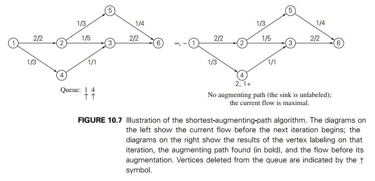
flows on them). In particular, for the network in Figure 10.7, the algorithm
finds the cut {(1, 2),
(4, 3)} of minimum capacity 3, both edges of which are
full as required.
Edmonds and Karp proved in
their paper [Edm72] that the number of aug-menting paths needed by the
shortest-augmenting-path algorithm never exceeds nm/2, where n and m
are the number of vertices and edges, respectively. Since the time required to find a shortest augmenting
path by breadth-first search is in O(n + m) = O(m) for networks represented by
their adjacency lists, the time efficiency of the shortest-augmenting-path
algorithm is in O(nm2).
More efficient algorithms for
the maximum-flow problem are known (see the monograph [Ahu93], as well as
appropriate chapters in such books as [Cor09] and [Kle06]). Some of them
implement the augmenting-path idea in a more efficient manner. Others are based
on the concept of preflows. A preflow is a flow that satisfies the
capacity constraints but not the flow-conservation requirement. Any vertex is
allowed to have more flow entering the vertex than leaving it. A preflow-push
algorithm moves the excess flow toward the sink until the flow-conservation
requirement is reestablished for all intermediate vertices of the network.
Faster al-gorithms of this kind have worst-case efficiency close to O(nm). Note that preflow-push algorithms fall outside
the iterative-improvement paradigm because they do not generate a sequence of
improving solutions that satisfy all
the constraints of the problem.
To conclude this section, it
is worth pointing out that although the initial interest in studying network
flows was caused by transportation applications, this model has also proved to
be useful for many other areas. We discuss one of them in the next section.
Exercises 10.2
Since maximum-flow algorithms require processing edges in both
directions, it is convenient to modify the adjacency matrix representation of a
network as follows. If there is a directed edge from vertex i to vertex j of capacity uij , then the element in the ith row and the j th column is set to uij , and the element in the j th row and the ith column is set to −uij ; if there is no edge between vertices i and j , both these elements are set to zero. Outline
a simple algorithm for identifying a source and a sink in a network presented
by such a matrix and indicate its time efficiency.
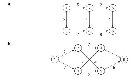
Apply the shortest-augmenting
path algorithm to find a maximum flow and a minimum cut in the following
networks.
a. Does the maximum-flow problem
always have a unique solution? Would your
answer be different for networks with different capacities on all their edges?
Answer the same questions for the minimum-cut problem of finding a
cut of the smallest capacity in a given network.
a. Explain how the maximum-flow
problem for a network with several sources
and sinks can be transformed into the same problem for a network with a single
source and a single sink.
Some networks have capacity constraints on the flow amounts that
can flow through their intermediate vertices. Explain how the maximum-flow
problem for such a network can be transformed to the maximum-flow problem for a
network with edge capacity constraints only.
Consider a network that is a rooted tree, with the root as its
source, the leaves as its sinks, and all the edges directed along the paths
from the root to the leaves. Design an efficient algorithm for finding a
maximum flow in such a network. What is the time efficiency of your algorithm?
a. Prove equality (10.9).
Prove that for any flow in a network and any cut in it, the value
of the flow is equal to the flow across the cut (see equality (10.12)). Explain
the relationship between this property and equality (10.9).
a. Express the maximum-flow
problem for the network in Figure 10.4 as a
linear programming problem.
Solve this linear programming problem by the simplex method.
As an alternative to the shortest-augmenting-path algorithm,
Edmonds and Karp [Edm72] suggested the maximum-capacity-augmenting-path
algorithm, in which a flow is augmented along the path that increases the flow
by the largest amount. Implement both these algorithms in the language of your
choice and perform an empirical investigation of their relative efficiency.
Write a report
on a more
advanced maximum-flow algorithm
such as
(i) Dinitz’s algorithm, (ii)
Karzanov’s algorithm, (iii) Malhotra-Kamar-Maheshwari algorithm, or (iv)
Goldberg-Tarjan algorithm.
Dining problem Several families go out to
dinner together. To increase their social
interaction, they would like to sit at tables so that no two members of the
same family are at the same table. Show how to find a seating arrangement that
meets this objective (or prove that no such arrangement exists) by using a
maximum-flow problem. Assume that the dinner contingent has p families and that the ith family has ai members. Also assume that q tables are available and the j th table has a seating capacity of bj . [Ahu93]
Related Topics