Chapter: Mathematics (maths) : Solution of Equations and Eigenvalue Problems
Solution of Equations and Eigenvalue Problems
SOLUTION OF EQUATIONS AND EIGENVALUE PROBLEMS
1
Numerical solution of Non-Linear Equations
Method of false position
Newton Raphson Method
Iteration Method
2
System of Linear Equations
Gauss Elimination Method
Gauss Jordan Method
Gauss Jacobi Method
Gauss Seidel Method
3
Matrix Inversion
Inversion by Gauss Jordan Method
4
Eigen Value of a Matrix
Von Mise`s power method
Introduction
The problem of solving the equation is
of great importance in science and Engineering.
In this section, we deal with the various methods
which give a solution for the equation
Solution
of Algebraic and transcendental equations
The equation of the form f(x) =0 are
called algebraic equations if f(x) is purely a polynomial in x.For example: are
algebraic equations .
If f(x) also contains trigonometric, logarithmic,
exponential function etc. then the equation is known as transcendental
equation.
Methods for solving the equation
The following result helps us to locate
the interval in which the roots of
Method of false position.
Iteration method
Newton-Raphson method
Method of False position (Or)
Regula-Falsi method (Or) Linear interpolation method
In bisection method the interval is always divided into half. If a function changes sign over an interval, the function value at the mid-point is evaluated. In bisection method the interval from a to b into equal intervals ,no account is taken of the magnitude of .An alternative method that exploits this graphical insights is to join by a straight line.The intersection of this line with the X-axis represents an improved estimate of the root.The replacement of the curve by a straight line gives a “ the origin of the name ,method of false position ,or in Latin ,Regula falsi .It is also called the linear interpolation method.
Problems
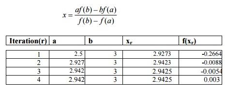
1. Find a real root of
that lies between 2 and 3 by the method of false position and correct
to three decimal places.
Sol:
Let
The
root lies between 2.5 and 3.
The
approximations are given by
2.
Obtain the real root of,correct to four decimal places using the method of
false position.
Sol:
Given
Taking logarithmic on both sides,
x log10 x 2
f (x) x log10
x 2
f (3.5)
0.0958 0 and f (3.6) 0.00027 0
The
roots lies between 3.5 and 3.6
The approximation are
given by
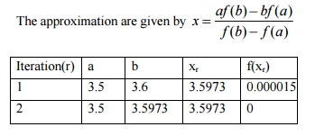
The required root is
3.5973
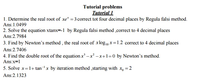
Exercise:
1. Determine the real
root of correct to four decimal places by Regula-Falsi method.
Ans: 1.0499
2. Find the positive
real root of correct to four decimals by the method of False position .
Ans: 1.8955
3.Solve the equation by
Regula-Falsi method,correct to 4 decimal places.
Ans: 2.7984
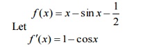
Newton’smethod(or) Newton-Raphson method
(Or) Method of tangents
This method starts with an initial
approximation to the root of an equation, a better and closer approximation to
the root can be found by using an iterative process.
Derivation of Newton-Raphson formula
Let be the root of f (x) 0 and x0 be an
approximation to .If hx0
Then
by the Tayor’s
series
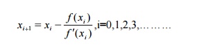
Note:
The error at any stage is proportional
to the square of the error in the previous stage.
The order of convergence of the
Newton-Raphson method is at least 2 or the convergence of N.R method is
Quadratic.
Problems
1.Using Newton’s method
,find the correct root five decimal between places.
Sol:
Given
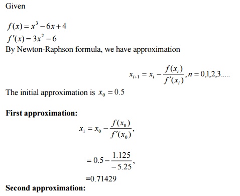
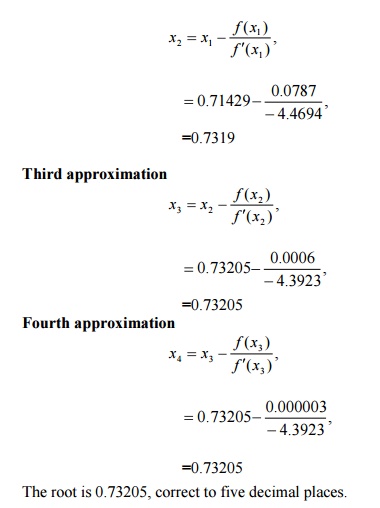
First approximation:=0.71429
Second approximation: 0.73109
The root is 0.73205, correct to five decimal places.
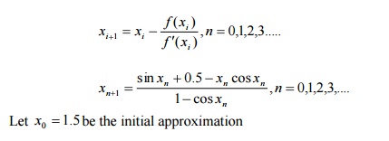
By Newton-Raphson formula, we have approximation
The initial approximation is x0 = 0.5
2. Find a real root of
x=1/2+sinx near 1.5, correct to 3 decimal places by newton-Rapson method. Sol:
By Newton-Raphson formula, we have approximation
First approximation:
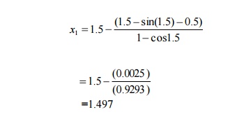
=1.497
Second approximation:
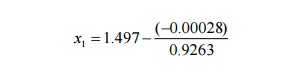
=1.497.
The required root is 1.497
Exercise:
1. Find the real root
of e x 3x ,that lies between 1 and 2 by New
places.
Ans:1.5121
2.Use Newton-Raphson method to solve the equation
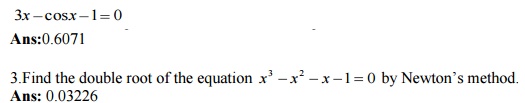
Ans: 0.03226
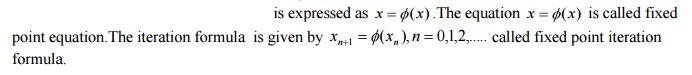
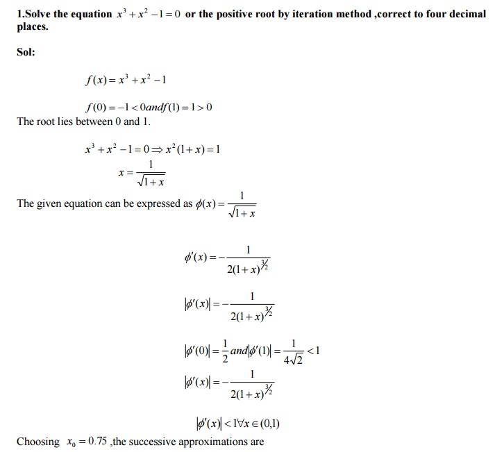
Iteration method (Or) Method of
successive approximations(Or)Fixed point method
For solving the equation f (x) = 0 by
iteration method, we start with an approximation value of the root.The
equation f (x)
Theorem(Fixed point theorem)
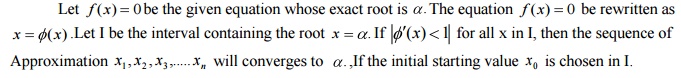
The order of convergence
Theorem

Note
The order of convergence in general is linear (i.e)
=1
Problems
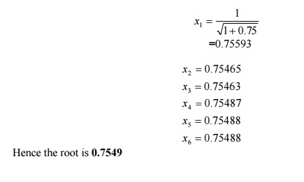
Hence the root is 0.7549
Exercise:
1. Find the cube root of 15, correct to four decimal
places, by iteration method
Ans: 2.4662
2 System of linear equation
Introduction
Many problems in
Engineering and science needs the solution of a system of simultaneous linear
equations .The solution of a system of simultaneous linear equations is
obtained by the following two types of methods
Direct methods (Gauss elimination and Gauss Jordan
method)
Indirect methods or iterative methods (Gauss Jacobi
and Gauss Seidel method)
(a) Direct methods are those in which
The computation can be completed in a finite number
of steps resulting in the exact solution
The amount of computation involved can be specified in advance.
The method is independent of the accuracy desired.
(b) Iterative methods (self correcting methods) are which
Begin with an approximate solution and
Obtain an improved solution with each step of
iteration
But would require an infinite number of steps to
obtain an exact solution without round-off errors
The accuracy of the solution depends on the number
of iterations performed.
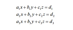
Simultaneous linear equations
The system of equations in n unknowns x1
, x2 , x3 ,..... xn is given by
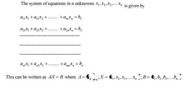
The system of equation can be solved by using determinants (Cramer’s rule) or by means of matrices.
These involve tedious calculations. These are other
methods to solve such equations .In this chapter we will discuss four methods
viz.
(i)
Gauss –Elimination method
(ii)
Gauss –Jordan method
(iii)
Gauss-Jacobi method
(iv)
Gauss seidel method
Ø
Gauss-Elimination method
This is an Elimination method and it reduces the
given system of equation to an equivalent upper triangular system which can be
solved by Back substitution.
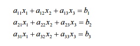
Consider the system of equations
Gauss-algorithm is explained below:
Step 1. Elimination
of x1 from the second and third equations .If
a11 != 0 the first equation is used to eliminate x1
from the second and third equation. After elimination, the reduced system is
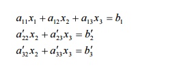
Step 2:
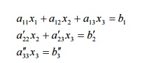
Elimination of x2 from the third equation. If a’22 != 0 We
eliminate x2 from third equation and the reduced upper
triangular system is
Step 3:
From third equation x3 is known. Using x3 in the second
equation x2 is obtained. using both x2
And x3 in the first equation,
the value of x1 is obtained.
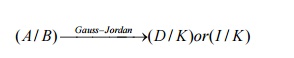
Thus the elimination method, we start with the
augmented matrix (A/B) of the given system and transform it to (U/K) by
eliminatory row operations. Finally the solution is obtained by back
substitution process.

2. Gauss –Jordan method
This method is a modification of Gauss-Elimination
method. Here the elimination of unknowns is performed not only in the equations
below but also in the equations above. The co-efficient matrix A of the system
AX=B is reduced into a diagonal or a unit matrix and the solution is obtained
directly without back substitution process.
Examples

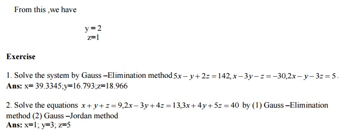
method (2) Gauss
–Jordan method Ans: x=1; y=3; z=5
Iterative method
These methods are used to solve a special of linear
equations in which each equation must possess one large coefficient and the
large coefficient must be attached to a different unknown in that
equation.Further in each equation, the absolute value of the large coefficient
of the unknown is greater than the sum of the absolute values of the other
coefficients of the other unknowns. Such type of simultaneous linear equations
can be solved by the following iterative methods.
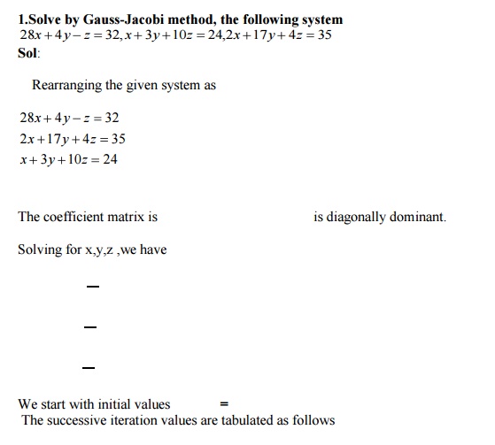
Gauss-Jacobi method
Gauss seidel method
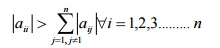
i.e., the co-efficient
matrix is diagonally dominant.
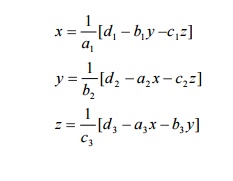
Solving the given system
for x,y,z (whose diagonals are the largest values),we have
Gauss-Jacobi method
If the rth iterates are x(r ) , y
(r ) , z (r )
,then the iteration scheme for this method is
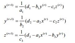
The
iteration is stopped when the values x, y, z start repeating with the desired
degree of accuracy.
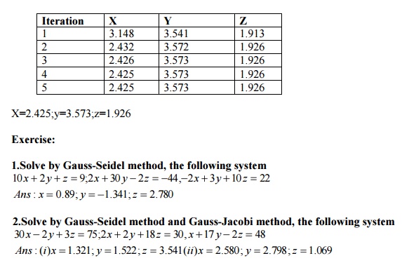
Gauss-Seidel method
This method is only a
refinement of Gauss-Jacobi method .In this method ,once a new value for a
unknown is found ,it is used immediately for computing the new values of the
unknowns.
If the rth iterates are, then the
iteration scheme for this method is
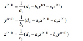
Hence finding the values of the unknowns, we use the
latest available values on the R.H.S The process of iteration is continued
until the convergence is obtained with desired accuracy.
Conditions for convergence
Gauss-seidel method will converge if in each
equation of the given system ,the absolute values o the largest coefficient is
greater than the absolute values of all the remaining coefficients
This is the sufficient condition for convergence of
both Gauss-Jacobi and Gauss-seidel iteration methods.
Rate of convergence
The rate of convergence
of gauss-seidel method is roughly two times that of Gauss-Jacobi method.
Further the convergences in Gauss-Seidel method is very fast in gauss-Jacobi
.Since the current values of the unknowns are used immediately in each stage of
iteration for getting the values of the unknowns.
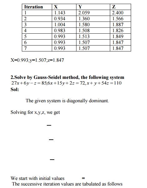
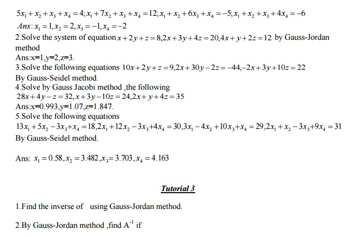
Problems
1.Solve by Gauss-Jacobi method, the
following system
3 Matrix inversion
Introduction
A square matrix whose
determinant value is not zero is called a non-singular matrix. Every non-singular
square matrix has an inverse matrix. In this chapter we shall find the inverse
of the non-singular square matrix A of order three. If X is the inverse of A,
Then
Inversion by Gauss-Jordan method
By Gauss Jordan method, the inverse matrix X is
obtained by the following steps:
Step 1: First consider the augmented matrix
Step 2: Reduce the matrix A in to the identity
matrix I by employing row transformations.
The row transformations used in step 2 transform I
to A-1
Finally write the inverse matrix A-1.so
the principle involved for finding A-1 is as shown below
Note
The
answer can be checked using the result
Problems
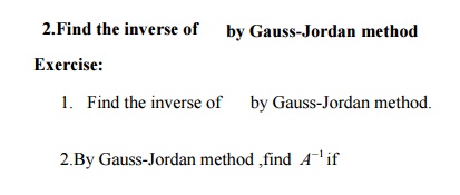
1.Find the inverse of by Gauss-Jordan
method.
4
Eigen value of a Matrix
Introduction
For every square matrix
A, there is a scalar λ and a non-zero column vector X such that AX= λ
X .Then the scalar λ is called an
Eigen value of A and X, the corresponding Eigen vector. We have studied earlier
the computation of Eigen values and the Eigen vectors by means of analytical
method. In this chapter, we will discuss an iterative method to determine the
largest Eigen value and the corresponding Eigen vector.
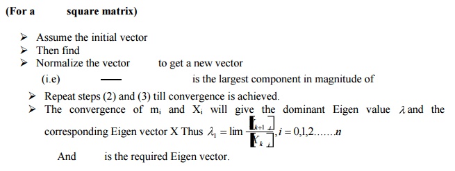
Power method (Von Mise’s power
method)
Power method is used to
determine numerically largest Eigen value and the corresponding Eigen vector of
a matrix A
Working Procedure
Problems
1.Use the power method
to find the dominant value and the corresponding Eigen vector of the matrix
Sol:
Let
--- - - ----
Hence the dominant Eigen value is 15.97 and the
corresponding Eigen vector is 2.
Determine the dominant Eigen value and the
corresponding Eigen vector of using
power method.
Exercise:
1. Find the dominant Eigen value and the
corresponding Eigen vector of A Find also the other two Eigen values.
2. Find the dominant Eigen value of the
corresponding Eigen vector of By power method. Hence find the other Eigen value
also.
|
Tutorial 2 |
|
|
1.Solve the following system by
Gauss-elimination method |
|
3.Determine the dominant Eigen value and the corresponding Eigen vector of using power method. Ans:[0.062,1,0.062]T
4.Find the smallest Eigen value and the corresponding Eigen vector of using power method. Ans:[0.707,1,0.707]T
5.Find the dominant Eigen value and the corresponding Eigen vector of by power method. Hence find the other Eigen value also . Ans:λ=2.381
Related Topics