Primal-Dual Relationships

PRIMAL-DUAL RELATIONSHIPS

Changes made in the original LP model will change the elements of the current optimal tableau, which in turn may affect the optimality and/or the feasibility of the cur-rent solution. This section introduces a number of primal-dual relationships that can be used to recompute the elements of the optimal simplex tableau. These relationships will form the basis for the economic interpretation of the LP model as well as for post-optimality analysis.

This section starts with a brief review of matrices, a convenient tool for carrying out the simplex tableau computations.

1. Review of Simple Matrix Operations

The simplex tableau computations (row use only three elementary matrix operations: vector) X (matrix), (matrix) x (column vector), and (scalar) X (matrix).These operations are summarized here for convenience. First, we introduce some matrix definitions:

1)    A matrix, A, of size (m X n) is a rectangular array of elements with m rows and n columns.

2)    A row vector, V, of size m is a (1 X  m) matrix.

3)    A column vector, P, of size n is an (n xl) matrix.

These definitions can be represented mathematically as

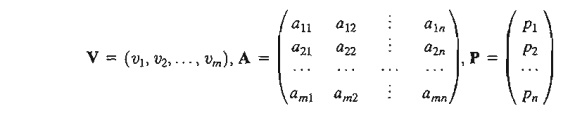
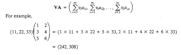
1. (Row vector X matrix, VA). The operation is defined only if the size of the row vector V equals the number of rows of A. In this case,

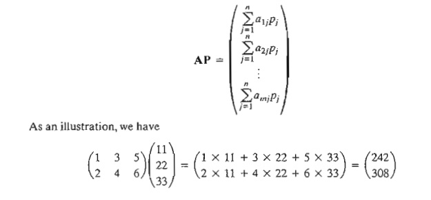
2. (Matrix X column vector, AP). The operation is defined only if the number of columns of A equals the size of column vector P. In this case,

3. (Scalar X matrix, aA). Given the scalar (or constant) quantity a, the multiplication operation aA will result in a matrix of the same size as A whose (i, j)th element equals aaij- For example, given a = 10,

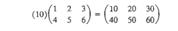
In general, aA = Aa. The same operation is extended equally to the multiplication of vectors by scalars. For example, aV = Va and aP = Pa.

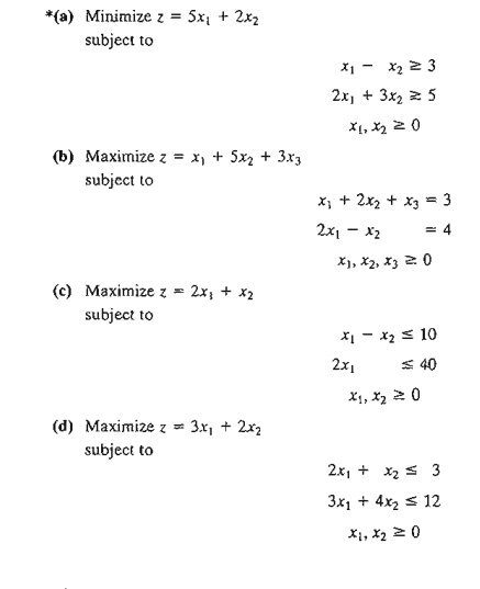
PROBLEM SET 4.2A

1. Consider the following matrices:

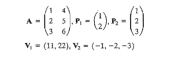
In each of the following cases, indicate whether the given matrix operation is legitimate, and, if so, calculate the result.

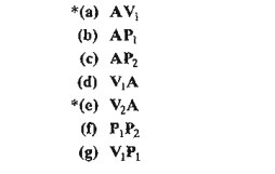
2. Simplex Tableau Layout

In Chapter 3, we followed a specific format for setting up the simplex tableau. This for-mat is the basis for the development in this chapter.

Figure 4.1 gives a schematic representation of the starting and general simplex tableaus. In the starting tableau, the constraint coefficients under the starting variables form an identity matrix (all main-diagonal elements equal 1 and all off-diagonal elements equal zero). With this arrangement, subsequent iterations of the simplex tableau generated by the Gauss-Jordan row operations (see Chapter 3) will modify the elements of the identity matrix to produce what is known as the inverse matrix. As we will see in the remainder of this chapter, the inverse matrix is key to computing all the elements of the associated simplex tableau.

PROBLEM SET 4.2B

1. Consider the optimal tableau of Example 3.3-1.

*(a) Identify the optimal inverse matrix.

(b) Show that the right-hand side equals the inverse multiplied by the original right-hand side vector of the original constraints.

2. Repeat Problem 1 for the last tableau of Example 3.4-1.

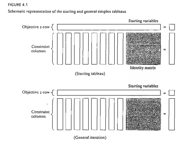
3. Optimal Dual Solution

The primal and dual solutions are so closely related that the optimal solution of either problem directly yields (with little additional computation) the optimal solution to the other. Thus, in an LP model in which the number of variables is considerably smaller than the number of constraints, computational savings may be realized by solving the dual, from which the primal solution is determined automatically. This result follows because the amount of simplex computation depends largely (though not totally) on the number of constraints (see Problem 2, Set 4.2c).

This section provides two methods for determining the dual values. Note that the dual of the dual is itself the primal, which means that the dual solution can also be used to yield the optimal primal solution automatically.

The elements of the row vector must appear in the same order in which the basic variables are listed in the Basic column of the simplex tableau.

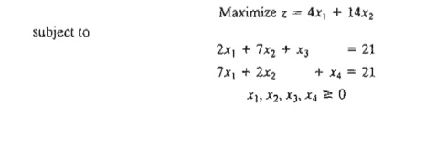
Example 4.2-1

Consider the following LP:

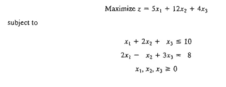
To prepare the problem for solution by the simplex method, we add a slack x₄ in the first constraint and an artificial R in the second. The resulting primal and the associated dual problems are thus defined as follows:

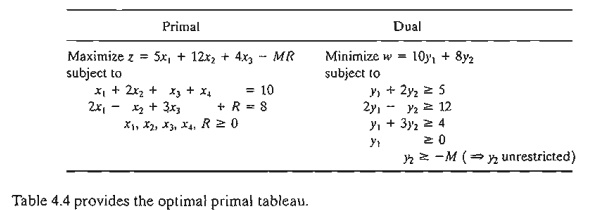
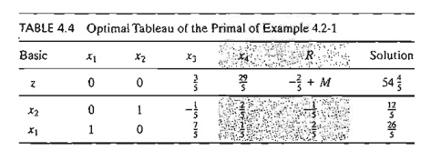
Table 4.4 provides the optimal primal tableau.

We now show how the optimal dual values are determined using the two methods described at the start of this section.

Method 1. In Table 4.4. the starting primal variables x₄ and R uniquely correspond to the dual variables y_l and y₂, respectively. Thus, we determine the optimum dual solution as follows:

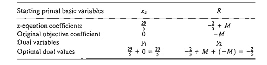
Method 2. The optimal inverse matrix, highlighted under the starting variables x4 and R, is given in Table 4.4 as

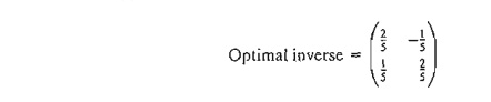
First, we note that the optimal primal variables are listed in the tableau in row order as x₂ and then x₁. This means that the elements of the original objective coefficients for the two variables must appear in the same order-namely,

(Original objective coefficients) =    (Coefficient of x₂, coefficient of x_I)

= (12,5)

TABLE 4.4 Optimal Tableau of the Primal of Example 4.2-1

Primal-dual objective values. Having shown how the optimal dual values are determined, next we present the relationship between the primal and dual objective values. For any pair ofjeasibLe primal and dual solutions,

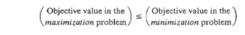
At the optimum, the relationship holds as a strict equation. The relationship does not specify which problem is primal and which is dual. Only the sense of optimization (maximization or minimization) is important in this case.

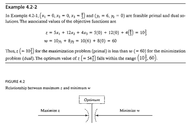
The optimum cannot occur with z strictly less than w (i.e., z < w) because, no matter how close z and ware, there is always room for improvement, which contradicts optimality as Figure 4.2 demonstrates.

PROBLEM SET 4.2C

1. Find the optimal value of the objective function for the following problem by inspecting only its dual. (Do not solve the dual by the simplex method.)

2. Solve the dual of the following problem, then find its optimal solution from the solution of the dual. Does the solution of the dual offer computational advantages over solving the primal directly?

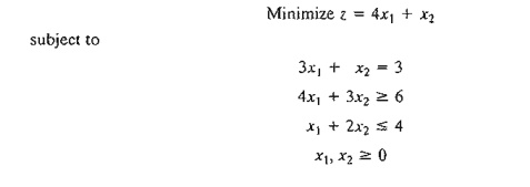
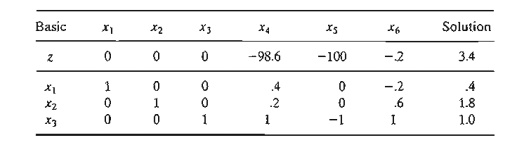
Given that the artificial variable x4 and the slack variable x5 form the starting basic variables and that M was set equal to 100 when solving the problem, the optimal tableau is given as

Write the associated dual problem and determine its optimal solution in two ways.

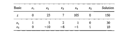
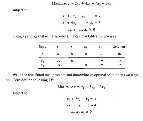
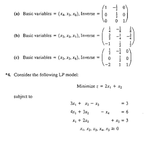
4. Consider the following LP: 

The starting solution consists of artificial x₄ and x₅ for the first and second constraints and slack x₆ for the third constraint. Using M = 100 for the artificial variables, the optimal tableau is given as

Write the associated dual problem and determine its optimal solution in two ways.

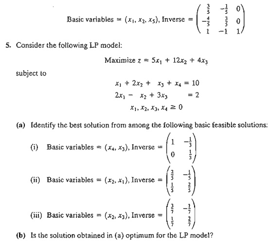
5. Consider the following LP:

The starting solution consists of x₃ in the first constraint and an artificial x₄ in the second constraint with M = 100. The optimal tableau is given as

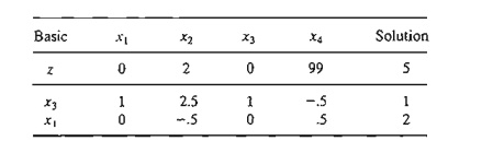
Write the associated dual problem and determine its optimal solution in two ways.

7. Consider the following set of inequalities:

A feasible solution can be found by augmenting the trivial objective function Maximize z = x₁ + x₂ and then solving the problem. Another way is to solve the dual; from which a solution for the set of inequalities can be found. Apply the two methods.

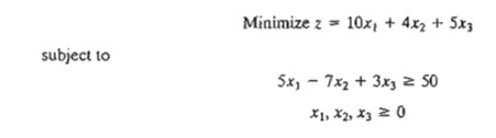
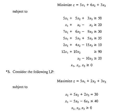
8. Estimate a range for the optimal objective value for the following LPs:

9. In Problem 7(a), let yl and y2 be the dual variables. Determine whether the following pairs of primal-dual solutions are optimal:

4. Simplex Tableau Computations

This section shows how any iteration of the entire simplex tableau can be generated from the original data of the problem, the inverse associated with the iteration, and the dual problem. Using the layout of the simplex tableau in Figure 4.1, we can divide the computations into two types:

a.   Constraint columns (Ieft- and right-hand sides).

b.  Objective z-row.

Formula 1: Constraint Column Computations. In any simplex iteration, a left-hand or a right-hand side column is computed as follows:

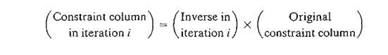
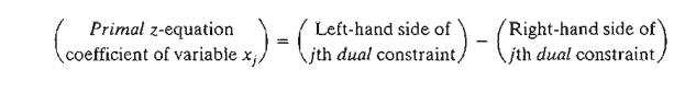
Formula 2: Objective z-row Computations. In any simplex iteration, the objective equation coefficient (reduced cost) of x_j is computed as follows:

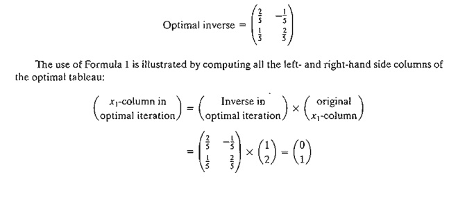
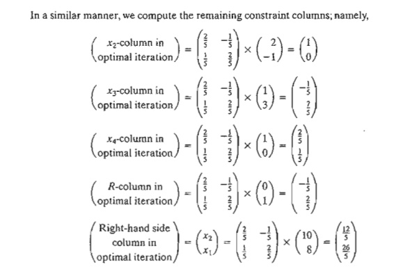
Example 4.2-3

We use the LP in Example 4.2-1 to illustrate the application of Formulas 1 and 2. From the optimal tableau in Table 4.4, we have

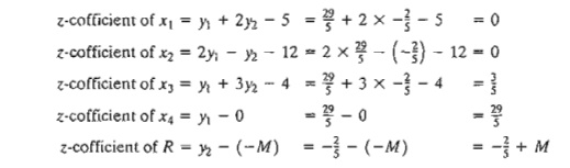
Next, we demonstrate how the objective row computations are carried out using Formula 2. The optimal values of the dual variables, (y₁. y₂) = (29/5,-2/5), were computed in Example 4.2-1 using two different methods. These values are used in Formula 2 to determine the associated z-coefficients; namely,

Notice that Formula 1 and Formula 2 calculations can be applied at any iteration of either the primal or the dual problems. All we need is the inverse associated with the (primal or dual) iteration and the original LP data.

PROBLEM SET 4.20

1. Generate the first simplex iteration of Example 4.2-1 (you may use TORA's Iterations => M-method for convenience), then use Formulas 1 and 2 to verify all the elements of the resulting tableau.

2. Consider the following LP model:

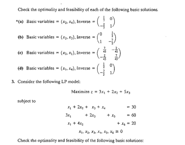
Compute the entire simplex tableau associated with the following basic solution and check it for optimality and feasibility.

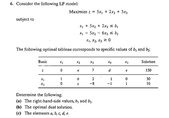
*7. The following is the optimal tableau for a maximization LP model with three (≤) constraints and all nonnegative variables. The variables x₃, x₄, and xs are the slacks associated with the three constraints. Determine the associated optimal objective value in two different ways by using the primal and dual objective functions.

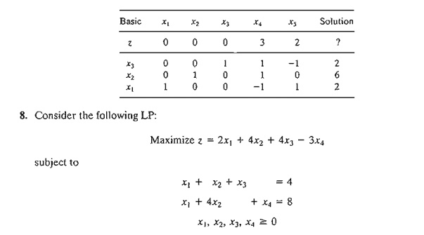
Use the dual problem to show that the basic solution (x₁, x₂)  is not optimal.

9. Show that Method 1 in Section 4.2.3 for determining the optimal dual values is actually based on the Formula 2 in Section 4.2.4.