Post-Optimal Analysis

POST-OPTIMAL ANALYSIS

In Section 3.6, we dealt with the sensitivity of the optimum solution by determining the ranges for the different parameters that would keep the optimum basic solution un-changed. In this section, we deal with making changes in the parameters of the model and finding the new optimum solution. Take, for example, a case in the poultry industry where an LP model is commonly used to determine the optimal feed mix per broiler (see Example 2.2-2). The weekly consumption per broiler varies from .26 lb (120 grams) for a one-week-old bird to 2.11b (950 grams) for an eight-week-old bird. Additionally, the cost of the ingredients in the mix may change periodically. These changes require periodic recalculation of the optimum solution. Post-optimal analysis deter-mines the new solution in an efficient way. The new computations are rooted in the use duality and the primal-dual relationships given in Section 4.2.

The following table lists the cases that can arise in post-optimal analysis and the actions needed to obtain the new solution (assuming one exists):

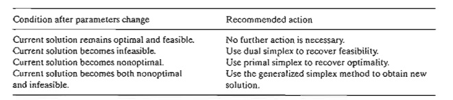
The first three cases are investigated in this section. The fourth case, being a combina-tion of cases 2 and 3, is treated in Problem 6, Set 4.5a.

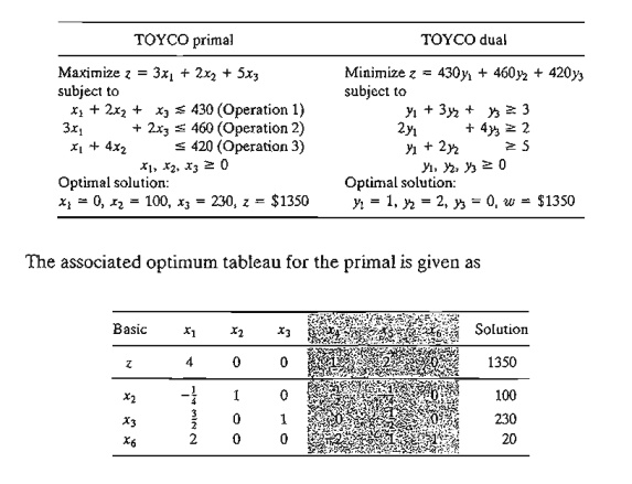
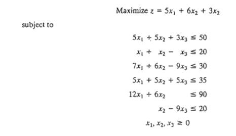
The TOYCO model of Example 4.3-2 will be used to explain the different procedures. Recall that the TOYCD model deals with the assembly of three types of. toys: trains, trucks, and cars. Three operations are involved in the assembly. We wish to determine the number of units of each toy that will maximize revenue. The model and its dual are repeated here for convenience.

1. Changes Affecting Feasibility

The feasibility of the current optimum solution may be affected only if (1) the right-hand side of the constraints is changed, or (2) a new constraint is added to the model. In both cases, infeasibility occurs when at least one element of the right-hand side of the optimal tableau becomes negative-that is, one or more of the current basic variables become negative.

Changes in the right-hand side. This change requires recomputing the right-hand side of the tableau using Formula 1 in Section 4.2.4:

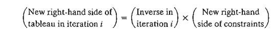
Recall that the right-hand side of the tableau gives the values of the basic variables.

Example 4.5-1

Situation 1. Suppose that TOYCO wants to expand its assembly lines by increasing the daily capacity of operations 1,2, and 3 by 40% to 602, 644, and 588 minutes, respectively. How would this change affect the total revenue?

With these increases, the only change that will take place in the optimum tableau is the right-hand side of the constraints (and the optimum objective value). Thus, the new basic solu-tion is computed as follows:

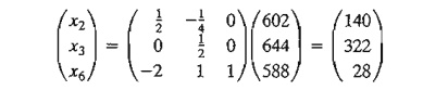
Thus, the current basic variables, x2, x3, and x6, remain feasible at the new values 140,322, and 28, respectively. The associated optimum revenue is $1890, which is $540 more than the cur-rent revenue of $1350.

Situation 2. Although the new solution is appealing from the standpoint of increased revenue, TOYCO recognizes that its implementation may take time. Another proposal was thus made to shift the slack capacity of operation 3 (x6 = 20 minutes) to the capacity of operation 1. How would this change impact the optimum solution?

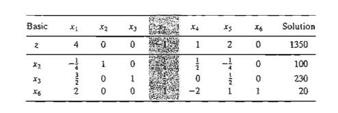
The capacity mix of the three operations changes to 450,460, and 400 minutes, respectively. The resulting solution is

The resulting solution is infeasible because x6 = -40, which requires applying the dual simplex method to recover feasibility. First, we modify the right-hand side of the tableau as shown by the shaded column. Notice that the associated value of z = 3 X 0 + 2 X 110 + 5 X 230 = $1370.

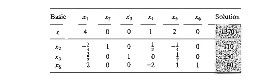
From the dual simplex, x6 leaves and x4 enters, which yields the following optimal feasible tableau (in general, the dual simplex may take more than one iteration to recover feasibility).

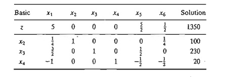
The optimum solution (in terms of x1, x2, and x3 ) remains the same as in the original model. This means that the proposed shift in capacity allocation is not advantageous in this- case because all it does is shift the surplus capacity in operation 3 to a surplus capacity in op-eration 1. The conclusion is that operation 2 is the bottleneck and it may be advantageous to shift the surplus to operation 2 instead (see Problem 1, Set 4.5a). The selection of operation 2 over operation 1 is also reinforced by the fact that the dual price for operation 2 ($2/min) is higher than that for operation 2 (= $l/min).

PROBLEM SET 4.5A

1. In the TOYCO model listed at the start of Section 4.5, would it be more advantageous to assign the 20-minute excess capacity of operation 3 to operation 2 instead of operation I?

2. Suppose that TOYCO wants to change the capacities of the three operations according to the following cases:

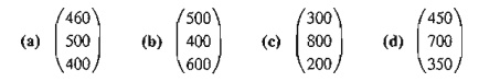
Use post-optimal analysis to determine the optimum solution in each case.

3. Consider the Reddy Mikks model of Example 2.1-1. Its optimal tableau is given in Exam-ple 3.3-1. If the daily availabilities of raw materials Ml and M2 are increased to 28 and 8 tons, respectively, use post-optimal analysis to determine the new optimal solution.

*4. The Ozark Farm has 20,000 broilers that are fed for 8 weeks before being marketed. The weekly feed per broiler varies according to the following schedule:

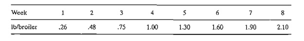
For the broiler to reach a desired weight gain in 8 weeks, the feedstuffs must satisfy specific nutritional needs. Although a typical list of feedstuffs is large, for simplicity we will limit the model to three items only: limestone, corn, and soybean meaL The nutritional needs will also be limited to three types: calcium, protein, and fiber. The following table summarizes the nutritive content of the selected ingredients together with the cost data.

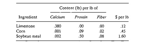
The feed mix must contain

a)     At least .8% but not more than 1.2% calcium

b)    At least 22% protein

c)     At most 5% crude fiber

Solve the LP for week 1 and then use post-optimal analysis to develop an optimal schedule for the remaining 7 weeks.

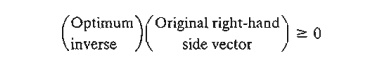
5. Show that the 100% feasibility rule in Problem 12, Set 3.6c (Chapter 3) is based on the condition

6. Post-optimal Analysis for Cases Affecting Both Optimality and Feasibility. Suppose that you are given the following simultaneous changes in the Reddy Mikks model: The revenue per ton of exterior and interior paints are $1000 and $4000, respectively, and the maximum daily availabilities of raw materials, M1 and M2, are 28 and 8 lons, respectively.

a.     Show that the proposed changes will render the current optimal solution both nonoptimal and infeasible.

b.     Use the generalized simplex algorithm (Section 4.4.2) to determine the new optimal feasible solution.

Addition of New Constraints. The addition of a new constraint to an existing model can lead to one of two cases.

a)     The new constraint is redundant, meaning that it is satisfied by the current opti-mum solution, and hence can be dropped from the model altogether.

b)    The current solution violates the new constraint, in which case the dual simplex method is used to restore feasibility.

Notice that the addition of a new constraint can never improve the current opti-mum objective value.

Example 4.5-3

Situation 1. Suppose that TOYCO is changing the design of its toys, and that the change will require the addition of a fourth operation in the assembly lines. The daily capacity of the new op-eration is 500 minutes and the times per unit for the three products on this operation are 3, 1, and 1 minutes, respectively. Study the effect of the new operation on the optimum solution.

The constraint for operation 4 is

3x1+x2+x3 ≤ 500

This constraint is redundant because it is satisfied by the current optimum solution xl ≤ 0, x2 ≤ 100, and x3 = 230. Hence, the current optimum solution remains unchanged.

Situation 2. Suppose, instead, that TOYCO unit times on the fourth operation are changed to 3, 3, and 1 minutes, respectively. All the remaining data of the model remain the same. Will the optimum solution change?

The constraint for operation 4 is

3x1+3x2+x3 ≤ 500

This constraint is not satisfied by the current optimum solution. Thus, the new constraint must be added to the current optimum tableau as follows (x7 is a slack):

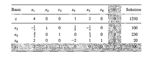
The tableau shows that x7 = 500, which is not consistent with the values of x2 and x3 in the rest of the tableau. The reason is that the basic variables x2 and x3 have not been substituted out in the new constraint. This substitution is achieved by performing the following operation:

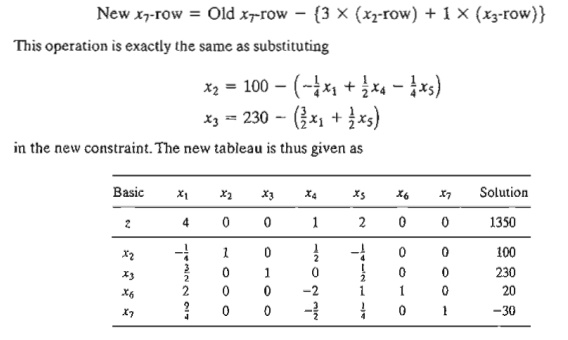
Application of the dual simplex method will produce the new optimum solution x1 = 0, x2 = 90, x3 = 230, and z = $1330 (verify!). The solution shows that the addition of operation 4 will worsen the revenues from $1350 to $1330.

PROBLEM SET 4.58

1. In the TOYCO model, suppose the fourth operation has the following specifications: The maximum production rate.based on 480 minutes a day is either 120 units of product 1, 480 units of product 2, or 240 units of product 3. Determine the optimal solution, assum-ing that the daily capacity is limited to

*(a) 570 minutes.

(b) 548 minutes.

2. Secondary Constraints. Instead of solving a problem using all of its constraints, we can start by identifying the so-called secondary constraints. These are the constraints that we suspect are least restrictive in terms of the optimum solution. The model is solved using the remaining (primary) constraints. We may then add the secondary constraints one at a time. A secondary constraint is discarded if it satisfies the available optimum. The process is repeated until all the secondary constraints are accounted for.

Apply the proposed procedure to the following LP:

2. Changes Affecting Optimality

This section considers two particular situations that could affect the optimality of the current solution:

a.   Changes in the original objective coefficients.

b.  Addition of a new economic activity (variable) to the model.

Changes in the Objective Function Coefficients.         These changes affect only the optimality of the solution. Such changes thus require recomputing the z-row coefficients (reduced costs) according to the following procedure:

a)     Compute the dual values using Method 2 in Section 4.2.3.

b)    Use the new dual values in Formula 2, Section 4.2.4, to determine the new re-duced costs (z-row coefficients).

Two cases will result:

1.     New z-row satisfies the optimality condition. The solution remains unchanged (the optimum objective value may change, however).

2.     The optimality condition is not satisfied. Apply the (primal) simplex method to recover optimality.

Example 4.5-4

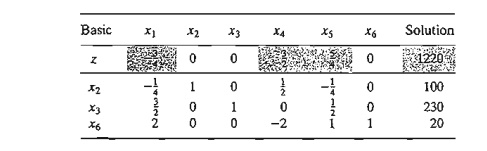
Situation 1. In the TOYCO model, suppose that the company has a new pricing policy to meet the competition. The unit revenues under the new policy are $2, $3, and $4 for train, truck, and car toys, respectively. How is the optimal solution affected?

The new objective function is

The z-row coefficients are determined as the difference between the left- and right-hand sides of the dual constraints (Fonnula 2, Section 4.2.4). It is not necessary to recompute the objective-row coefficients of the basic variables x2, x3, and x6 because they always equal zero regardless of any changes made in the objective coefficients (verify!).

Note that the right-hand side of the first dual constraint is 2, the new coefficient in the modified objective function.

The computations show that the current solution, x1 == 0 train, x2 = 100 trucks, and x3 = 230 cars, remains optimal. The corresponding new revenue is computed as 2 x 0 + 3 x 100 + 4 x 230 = $1220. The new pricing policy is not advantageous because it leads to lower revenue.

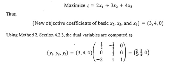
Situation 2.       Suppose now that the TOYCO objective function is changed to

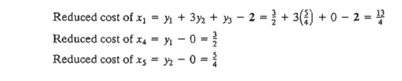
The new reduced cost of xl shows that the current solution is not optimum.

To determine the new solution, the z-row is changed as highlighted in the following tableau:

The elements shown in the shaded cells are the new reduced cost for the nonbasic variables x1, x4, and x5. All the remaining elements are the same as in the original optimal tableau. The new optimum solution is then determined by letting x1 enter and x6 leave, which yields xl = 10, x2 = 102.5, x3 = 215, and z = $1227.50 (verify!). Al-though the new solution recommends the production of all three toys, the optimum revenue is less than when two toys only are manufactured.

PROBLEM SET 4.5C

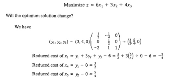
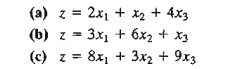
1. Investigate the optimality of the TOYCO solution for each of the following objective functions. If the solution changes, use post-optimal analysis to determine the new opti-mum. (The optimum tableau of TOYCO is given at the start of Section 4.5.)

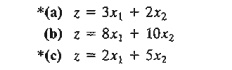
2. Investigate the optimality of the Reddy Mikks solution (Example 4.3-1) for each of the following objective functions. If the solution changes, use post-optimal analysis to deter-mine the new optimum. (The optimal tableau of the model is given in Example 3.3-1.)

3. Show that the 100% optimality rule (Problem 8, Set 3.6d, Chapter 3) is derived from (reduced costs) ≥ 0 for maximization problems and (reduced costs) ≤ 0 for minimization problems.

Addition of a New Activity. The addition of a new activity in an LP model is equivalent to adding a new variable. Intuitively, the addition of a new activity is desirable only if it is profitable-that is, if it improves the optimal value of the objective function. This condition can be checked by computing the reduced cost of the new variable using Formula 2, Section 4.2.4. If the new activity satisfies the optimality condition, then the activity is not profitable. Else, it is advantageous to undertake the new activity.

Example 4.5-5

TOYCO recognizes that toy trains are not currently in production because they are not prefitabre. The company wants to replace toy trains with a new product, a toy fire engine, to be assembled on the existing facilities. TOYCO estimates the revenue per toy fire engine to be $4 and the assembly times per unit to be 1 minute on each of operations 1 and 2, and 2 minutes on operation 3. How would this change impact the solution?

Let x7 represent the new fire engine product. Given that (y1, y2, y3 ) = (1,2,0) are the optimal dual values, we get

The result shows that it is profitable to include x7 in the optimal basic solution. To obtain the new optimum, we first compute its column constraint using Formula 1, Section 4.2.4, as

The new optimum is determined by letting x7 enter the basic solution, in which case x6 must leave. The new solution is x1 = 0, x2 = 0, x3 = 125, x7 = 210, and z = $1465 (verify!), which improves the revenues by $115.

PROBLEM SET 4.50

*1. In the original TOYCO model, toy trains are not part of the optimal product mix. The company recognizes that market competition will not allow raising the unit price of the toy. Instead, the company wants to concentrate on improving the assembly operation it-self. This entails reducing the assembly time per unit in each of the three operations by a specified percentage, p%. Determine the value of p that will make toy trains just prof-itable. (The optimum tableau of the TOYCO model is given at the start of Section 4.5.)

2. In the TOYCO model, suppose that the company can reduce the unit times on operations 1,2, and 3 for toy trains from the current levels of 1,3, and 1 minutes to .5,1, and .5 min-utes, respectively. The revenue per unit remains unchanged at $3. Determine the new op-timum solution.

3. In the TOYCO model, suppose that a new toy (fire engine) requires 3, 2, 4 minutes, re-spectively, on operations 1,2, and 3. Determine the optimal solution when the revenue per unit is given by

*(a) $5.

(b) $10.

4. In the Reddy Mikks model, the company is considering the production of a cheaper brand of exterior paint whose input requirements per ton include .75 ton of each of raw materials Ml and M2. Market conditions still dictate that the excess of interior paint over the production of both types of exterior paint be limited to 1 ton daily. The revenue per ton of the new exterior paint is $3500. Determine the new optimal solution. (The model is explained in Example 4.5-1, and its optimum tableau is given in Example 3.3-1.)