Economic Interpretation of Duality

ECONOMIC INTERPRETATION OF DUALITY

The linear programming problem can be viewed as a resource allocation model in which the objective is to maximize revenue subject to the availability of limited re-sources. Looking at the problem from this standpoint, the associated dual problem of-fers interesting economic interpretations of the LP resource allocation model.

To formalize the discussion, we consider the following representation of the gen-eral primal and dual problems:

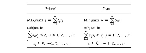
Viewed as a resource allocation model, the primal problem has n economic activities and m resources. The coefficient Cj in the primal represents the revenue per unit ofactivity j. Resource i, whose maximum availability is b_i , is consumed at the rate aij units per unit of activity j.

1. Economic Interpretation of Dual Variables

Section 4.2.3 states that for any two primal and dual feasible solutions, the values of the objective functions, when finite, must satisfy the following inequality:

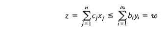
The strict equality, z =  w, holds when both the primal and dual solutions are optimal. Let us consider the optimal condition z = w first. Given that the primal problem represents a resource allocation model, we can think of z as representing revenue dollars. Because b_i  represents the number of units available of resource i, the equation

z =  w can be expressed dimensionally as

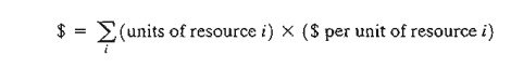
This means that the dual variable, y_i  represents the worth per unit of resource i. As stated in Section 3.6, the standard name dual (or shadow) price of resource i replaces the name worth per unit in all LP literature and software packages.

Using the same logic, the inequality z < w associated with any two feasible pri-mal and dual solutions is interpreted as

(Revenue) < (Worth of resources)

This relationship says that so long as the total revenue from all the activities is less than the worth of the resources, the corresponding primal and dual solutions are not opti-mal. Optimality (maximum revenue) is reached only when the resources have been ex-ploited completely, which can happen only when the input (worth of the resources) equals the output (revenue dollars). In economic terms, the system is said to be unstable (nonoptimal) when the input (worth of the resources) exceeds the output (revenue). Stability occurs only when the two quantities are equal.

Example 4.3-1

The Reddy Mikks model (Example 2.1-1) and its dual are given as:

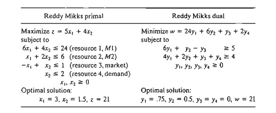
Briefly, the Reddy Mikks model deals with the production of two types of paint (interior and exterior) using two raw materials Ml and M2 (resources 1 and 2) and subject to market and demand limits represented by the third and fourth constraints. The model determines the amounts (in tons/day) of interior and exterior paints that maximize the daily revenue (expressed in thousands of dollars).

The optimal dual solution shows that the dual price (worth per unit) of raw material Ml (re-source 1) is y_l = .75 (or $750 per ton), and that of raw material M2 (resource 2) is y₂ = .5 (or $500 per ton). These results hold true for specific feasibility ranges as we showed in Section 3.6. For resources 3 and 4, representing the market and demand limits, the dual prices are both zero, which indicates that their associated resources are abundant. Hence, their worth per unit is zero.

PROBLEM SET 4.3A

1. In Example 4.3-1, compute the change in the optimal revenue in each of the following cases (use TORA output to obtain the feasibility ranges):

a.   The constraint for raw material M1 (resource 1) is 6x_l  + 4x₂  ≤ 22.

b.     The constraint for raw material M2 (resource 2) is x₁  + 2x₂ ≤  4.5.

c.      The market condition represented by resource 4 is x₂  ≤ 10.

*2. NWAC Electronics manufactures four types of simple cables for a defense contractor. Each cable must go through four sequential operations: splicing, soldering, sleeving, and inspection. The following table gives the pertinent data of the situation.

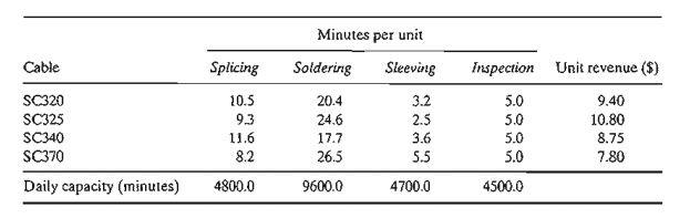
The contractor guarantees a minimum production level of 100 units for each of the four cables.

a.     Formulate the problem as a linear programming model, and determine the optimum production schedule.

b.     Based on the dual prices, do you recommend making increases in the daily capacities of any of the four operations? Explain.

c.      Does the minimum production requirements for the four cables represent an advan-tage or a disadvantage for NWAC Electronics? Provide an explanation based on the dual prices.

d.     Can the present unit contribution to revenue as specified by the dual price be guar-anteed if we increase the capacity of soldering by 1O%?

3. BagCo produces leather jackets and handbags. A jacket requires 8 m² of leather, and a handbag only 2 m²• The labor requirements for the two products are 12 and 5 hours, re-spectively. The current weekly supplies of leather and labor are limited to 1200 m² and 1850 hours. The company sells the jackets and handbags at $350 and $120, respectively. The objective is to determine the production schedule that maximizes the net revenue. BagCo is considering an expansion of production. What is the maximum purchase price The company should pay for additional leather? For additional labor?

2. Economic Interpretation of Dual Constraints

The dual constraints can be interpreted by using Formula 2 in Section 4.2.4, which states that at any primal iteration,

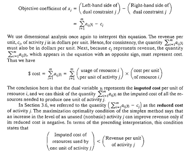
The maximization optimality condition thus says that it is economically advantageous to increase an activity to a positive level if its unit revenue exceeds its unit imputed cost.

We will use the TOYCO model of Section 3.6 to demonstrate the computation. The details of the model are restated here for convenience.

Example 4.3-2

TOYCO assembles three types of toys: trains, trucks, and cars using three operations. Available assembly times for the three operations are 430,460, and 420 minutes per day, respectively, and the revenues per toy train, truck, and car are $3, $2, and $5, respectively. The assembly times per train for the three operations are 1,3, and 1 minutes, respectively. The corresponding times per truck and per car are (2,0,4) and (1,2,0) minutes (a zero time indicates that the operation is not used).

Letting x₁,x₂,and x₃ represent the daily number of units assembled of trains, trucks and cars, the associated LP model and its dual are given as:

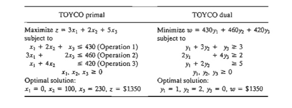
The optimal primal solution calls for producing no toy trains, 100 toy trucks, and 230 toy cars. Suppose that TOYCO is interested in producing toy trains as well. How can this be achieved? Looking at the problem from the standpoint of the interpretation of the reduced cost for xl> toy trains will become attractive economically only if the imputed cost of the resources used to produce one toy train is strictly less than its unit revenue. TOYCO thus can either in-crease the unit revenue per unit by raising the unit price, or it can decrease the imputed cost of the used resources (= y₁ + 3y₂ + y₃). An increase in unit price may not be possible because of market competition. A decrease in the unit imputed cost is more plausible because it entails making improvements in the assembly operations. Letting r₁, r₂, and r₃ represent the propor-tions by which the unit times of the three operations are reduced, the problem requires deter-mining r₁, r₂, and r3 such that the new imputed cost per per toy train is less than its unit revenue-that is,

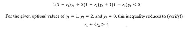
Thus, any values of r₁ and r₂ between 0 and 1 that satisfy r₁ + 6r₂ > 4 should make toy trains profitable. However, this goal may not be achievable because it requires practically impossible reductions in the times of operations 1 and 2. For example, even reductions as high as 50% in these times (that is, r_l = r₂ = .5) fail to satisfy the given condition. Thus, TOYCO should not produce toy trains unless an increase in its unit price is possible.

PROBLEM SET 4.3B

1. In Example 4.3-2, suppose that for toy trains the per-unit time of operation 2 can be reduced from 3 minutes to at most 1.25 minutes. By how much must the per-unit time of operation 1 be reduced to make toy trains just profitable?

*2. In Example 4.3-2, suppose that TOYCO is studying the possibility of introducing a fourth toy: fire trucks. The assembly does not make use of operation 1. Its unit assembly times on operations 2 and 3 are 1 and 3 minutes, respectively. The revenue per unit is $4. Would you advise TOYCO to introduce the new product?

*3. JoShop uses lathes and drill presses to produce four types of machine parts, PPl, PP2, PP3, and PP4. The table below summarizes the pertinent data.

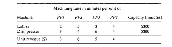
For the parts that are not produced by the present optimum solution, determine the rate of deterioration in the optimum revenue per unit increase of each of these products.

4. Consider the optimal solution of JoShop in Problem 3. The company estimates that for each part that is not produced (per the optimum solution), an across-the-board 20% re. duction in machining time can be realized through process improvements. Would these improvements make these parts profitable? If not, what is the minimum percentage re-duction needed to realize revenueability?