Methods of finding initial Basic Feasible Solutions: Vogel’s Approximation Method(VAM)

Methods of finding initial Basic Feasible Solutions

There are several methods available to obtain an initial basic feasible solution of a transportation problem. We discuss here only the following three. For finding the initial basic feasible solution total supply must be equal to total demand.

Method: Vogel’s Approximation Method(VAM)

Vogel’s approximation method yields an initial basic feasible solution which is very close to the optimum solution.Various steps involved in this method are summarized as under

Step 1: Calculate the penalties for each row and each column. Here penalty means the difference between the two successive least cost in a row and in a column .

Step 2: Select the row or column with the largest penalty.

Step 3: In the selected row or column, allocate the maximum feasible quantity to the cell with the minimum cost.

Step 4: Eliminate the row or column where all the allocations are made.

Step 5: Write the reduced transportation table and repeat the steps 1 to 4.

Step 6: Repeat the procedure until all the allocations are made.

Example 10.5

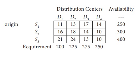
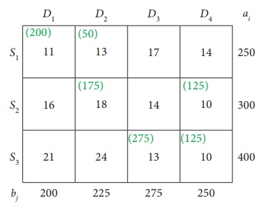
Find the initial basic feasible solution for the following transportation problem by VAM

Solution:

Here ∑ai = ∑bj = 950

(i.e) Total Availability =Total Requirement

∴The given problem is balanced transportation problem.

Hence there exists a feasible solution to the given problem.

First let us find the difference (penalty) between the first two smallest costs in each row and column and write them in brackets against the respective rows and columns

Choose the largest difference. Here the difference is 5 which corresponds to column D1 and D2. Choose either D1 or D2 arbitrarily. Here we take the column D1 . In this column choose the least cost. Here the least cost corresponds to (S1, D1) . Allocate min (250, 200) = 200units to this Cell.

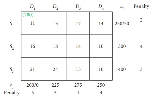
The reduced transportation table is

Choose the largest difference. Here the difference is 5 which corresponds to column D2. In this column choose the least cost. Here the least cost corresponds to (S1, D2) . Allocate min(50,175) = 50 units to this Cell.

The reduced transportation table is

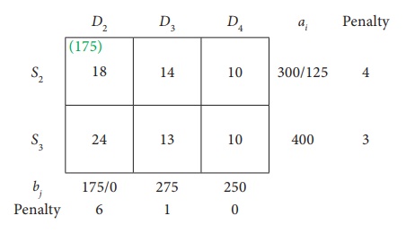
Choose the largest difference. Here the difference is 6 which corresponds to column D2. In this column choose the least cost. Here the least cost corresponds to (S2, D2) .

Allocate min(300,175) = 175 units to this cell.

The reduced transportation table is

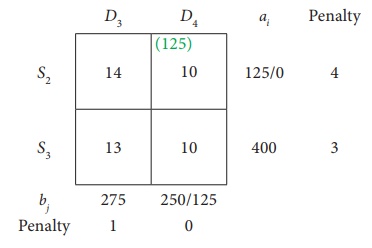
Choose the largest difference. Here the difference is 4 corresponds to row S2. In this row choose the least cost. Here the least cost corresponds to (S2, D4) . Allocate min(125,250) = 125 units to this Cell.

The reduced transportation table is 

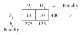
The Allocation is

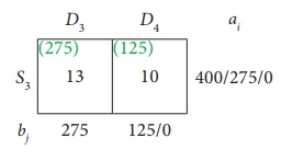
Thus we have the following allocations:

Transportation schedule :

S1→ D1, S1→D2, S2→D2, S2→D4, S3→D3, S3→D4

This initial transportation cost

= (200 × 11) + (50 ×13) + (175 × 18) + (125 ×10) + (275 ×13) + (125 ×10)

=  â‚¹ 12,075

Example 10.5

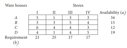
Obtain an initial basic feasible solution to the following transportation problem using Vogel’s approximation method.

Solution:

Here ∑ai = ∑bj = 80 (i.e) Total Availability =Total Requirement

∴The given problem is balanced transportation problem.

Hence there exists a feasible solution to the given problem.

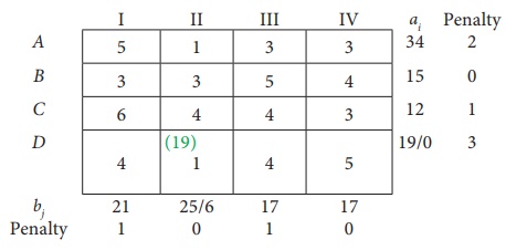
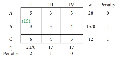
First Allocation:

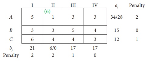
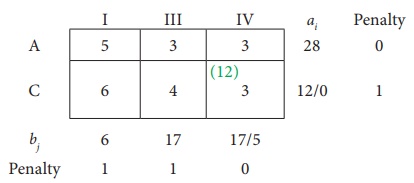
Second Allocation:

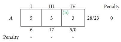
Third Allocation:

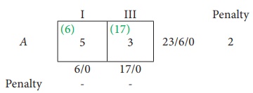
Fourth Allocation:

Fifth Allocation:

Sixth Allocation:

Thus we have the following allocations:

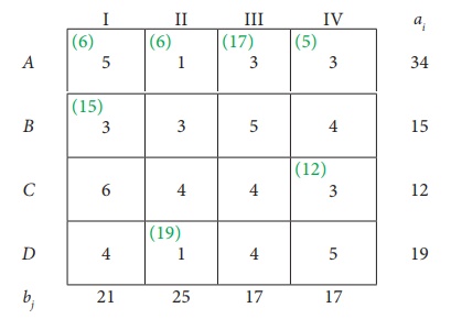
Transportation schedule :

A→ I, A→II, A→III, A→IV, B→I, C→IV, D→II

Total transportation cost:

= ( 6 × 5)+ ( 6 + 1)+ (17 × 3)+ ( 5 × 3)+ (15 × 3) + (12 × 3)+ (1 9 ×1)

= 30 + 6 + 51 + 15 + 45 + 36 + 19

= ₹ 202