Magnetostatics

Magnetostatics

In previous chapters we have seen that an electrostatic field is produced by static or stationary charges. The relationship of the steady magnetic field to its sources is much more complicated.

The source of steady magnetic field may be a permanent magnet, a direct current or an electric field changing with time. In this chapter we shall mainly consider the magnetic field produced by a direct current. The magnetic field produced due to time varying electric field will be discussed later. Historically, the link between the electric and magnetic field was established Oersted in 1820. Ampere and others extended the investigation of magnetic effect of electricity

. There are two major laws governing the magnetostatic fields are:

·           Biot-Savart Law

·           Ampere's Law

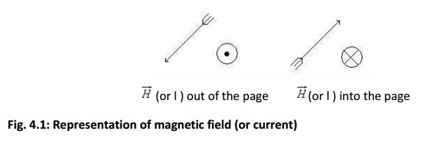
ually, the magnetic field intensity is represented by the vector H(Bar). It is customary to represent the direction of the magnetic field intensity (or current) by a small circle with a dot or cross sign depending on whether the field (or current) is out of or into the page as shown in Fig. 4.1.

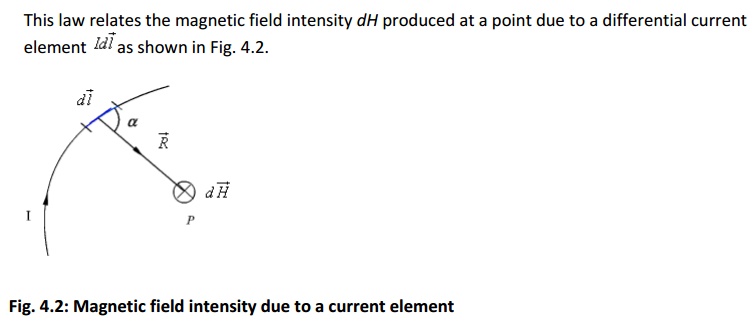
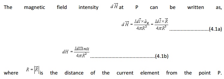
Biot- Savart Law

Similar to different charge distributions, we can have different current distribution such as line current, surface current and volume current. These different types of current densities are shown in Fig. 4.3.

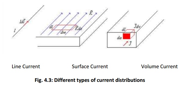
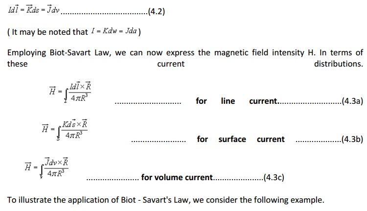
By denoting the surface current density as K (in amp/m) and volume current density as J (in amp/m2) we can write:

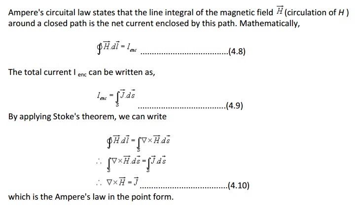
Ampere's Circuital Law:

Applications of Ampere's law:

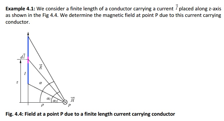
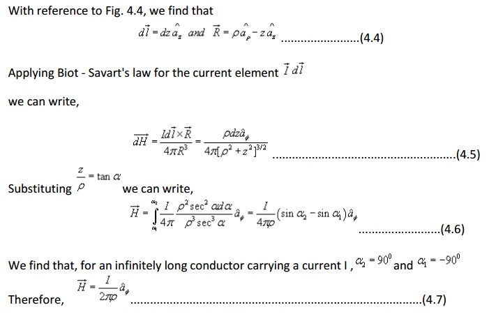
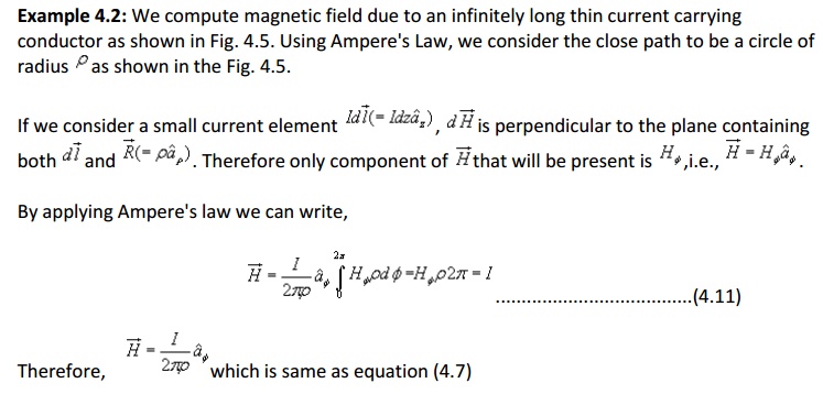
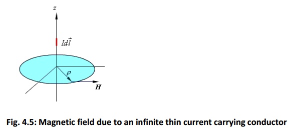
We illustrate the application of Ampere's Law with some examples.

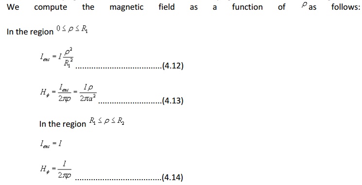
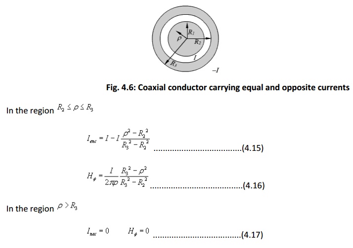
Example 4.3: We consider the cross section of an infinitely long coaxial conductor, the inner conductor carrying a current I and outer conductor carrying current - I as shown in figure 4.6.

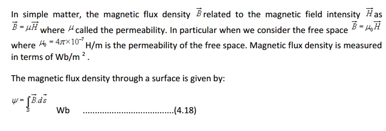
Magnetic Flux Density: 

In the case of electrostatic field, we have seen that if the surface is a closed surface, the net flux passing through the surface is equal to the charge enclosed by the surface. In case of magnetic field isolated magnetic charge (i. e. pole) does not exist. Magnetic poles always occur in pair (as N-S). For example, if we desire to have an isolated magnetic pole by dividing the magnetic bar successively into two, we end up with pieces each having north (N) and south (S) pole as shown in Fig. 4.7 (a). This process could be continued until the magnets are of atomic dimensions; still we will have N-S pair occurring together. This means that the magnetic poles cannot be isolated.

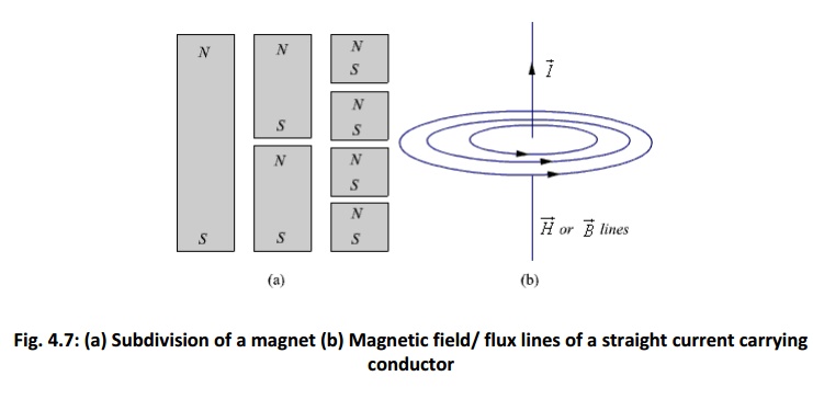
Similarly if we consider the field/flux lines of a current carrying conductor as shown in Fig. 4.7 (b), we find that these lines are closed lines, that is, if we consider a closed surface, the number of flux lines that would leave the surface would be same as the number of flux lines that would enter the surface.

From our discussions above, it is evident that for magnetic field,

which is the Gauss's law for the magnetic field.

By applying divergence theorem, we can write:

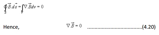
which is the Gauss's law for the magnetic field in point form.

Magnetic Scalar and Vector Potentials:

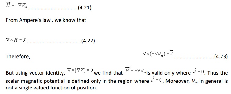
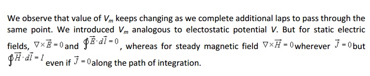
In studying electric field problems, we introduced the concept of electric potential that simplified the computation of electric fields for certain types of problems. In the same manner let us relate the magnetic field intensity to a scalar magnetic potential and write:

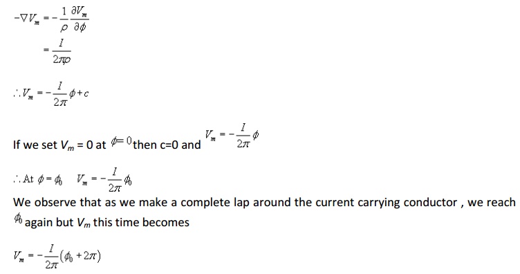
This point can be illustrated as follows. Let us consider the cross section of a coaxial line as shown in fig 4.8.

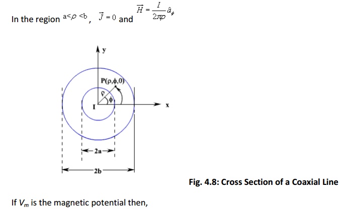
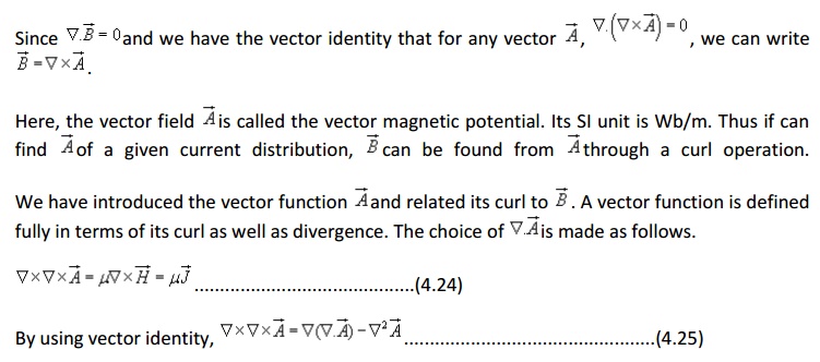
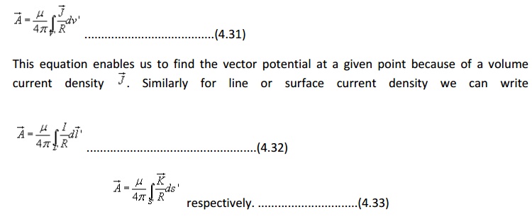
We now introduce the vector magnetic potential which can be used in regions where current density may be zero or nonzero and the same can be easily extended to time varying cases. The use of vector magnetic potential provides elegant ways of solving EM field problems.

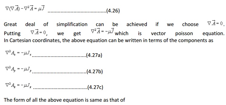
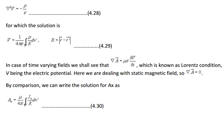
Computing similar solutions for other two components of the vector potential, the vector potential can be written as

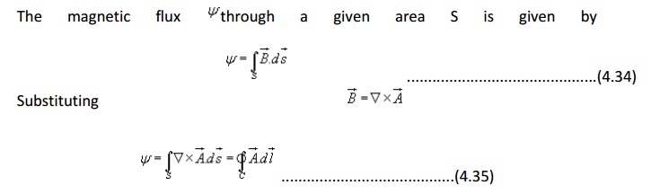
Vector potential thus have the physical significance that its integral around any closed path is equal to the magnetic flux passing through that path.

Boundary Condition for Magnetic Fields:

Similar to the boundary conditions in the electro static fields, here we will consider the

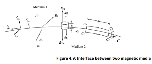
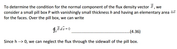
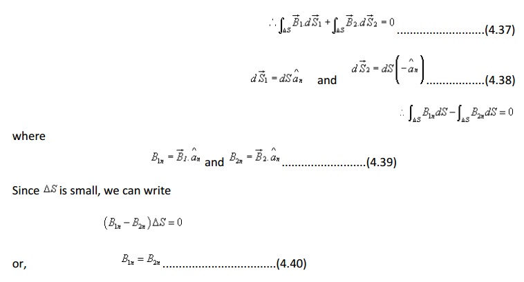
That is, the normal component of the magnetic flux density vector is continuous across the interface.

In vector form,

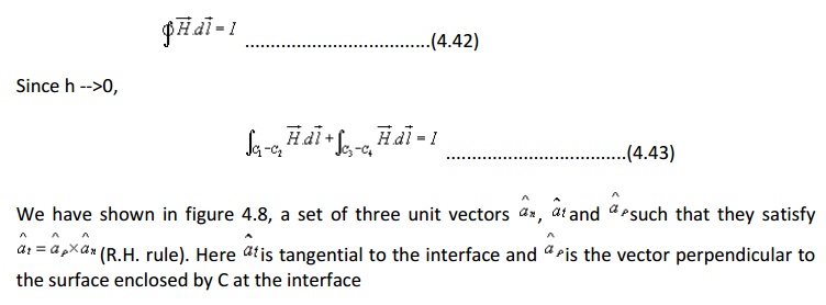
To determine the condition for the tangential component for the magnetic field, we consider a closed path C as shown in figure 4.8. By applying Ampere's law we can write

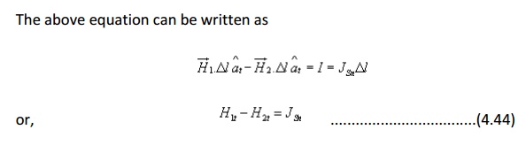
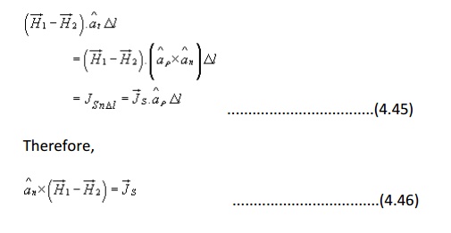
i.e., tangential component of magnetic field component is discontinuous across the interface where a free surface current exists.

If Js = 0, the tangential magnetic field is also continuous. If one of the medium is a perfect conductor Js exists on the surface of the perfect conductor.

In vector form we can write,

ASSIGNMENT PROBLEMS

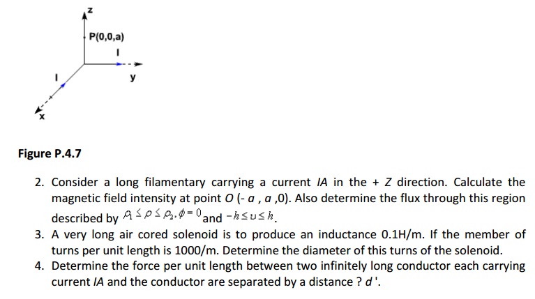
1. An infinitely long conductor carries a current I A is bent into an L shape and placed as shown in Fig. P.4.7. Determine the magnetic field intensity at a point P (0,0, a).