Linear Regression and Calibration Curves

Linear Regression and Calibration Curves

In a single-point external standardization, we first determine the value of k by measuring the signal for a single standard containing a known concentration of analyte. This value of k and the signal for the sample are then used to calculate the concentration of analyte in the sample (see Example 5.2). With only a single determination of k, a quantitative analysis using a single-point external stan- dardization is straightforward. This is also true for a single-point standard addi- tion (see Examples 5.4 and 5.5) and a single-point internal standardization (see Example 5.8).

A multiple-point standardization presents a more difficult problem. Consider the data in Table 5.1 for a multiple-point external standardiza- tion. What is the best estimate of the relationship between S_meas and C_S? It is tempting to treat this data as five separate single-point standardizations, determining k for each stan- dard and reporting the mean value. Despite its simplicity, single-point standardizations, determining k for each stan dard and reporting the mean value. Despite its simplicity, this is not an appropriate way to treat a multiple-point standardization.

In a single-point standardization, we assume that the reagent blank (the first row in Table 5.1) corrects for all constant sources of determinate error. If this is not the case, then the value of k determined by a single- point standardization will have a determinate error.

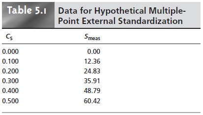
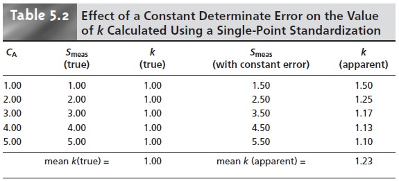
Table 5.2 demonstrates how an uncorrected constant error affects our determination of k. The first three columns show the concentration of analyte, the true measured signal (no constant error) and the true value of k for five standards. As expected, the value of k is the same for each standard. In the fourth column a constant determinate error of +0.50 has been added to the measured signals. The corresponding val- ues of k are shown in the last column. Note that a different value of k is obtained for each standard and that all values are greater than the true value. As we noted, this is a significant limitation to any single-point standardization.

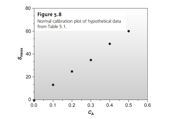
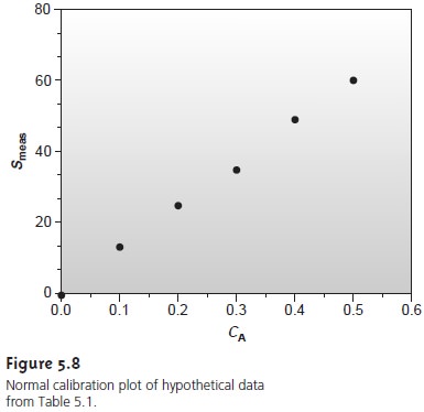
How do we find the best estimate for the relationship be- tween the measured signal and the concentration of analyte in a multiple-point standardization? Figure 5.8 shows the data in Table 5.1 plotted as a normal calibration curve. Although the data appear to fall along a straight line, the actual calibration curve is not intuitively obvious. The process of mathemati- cally determining the best equation for the calibration curve is called regression.

Linear Regression of Straight-Line Calibration Curves

A calibration curve shows us the relationship between the measured signal and the analyte’s concentration in a series of standards. The most useful calibration curve is a straight line since the method’s sensitivity is the same for all concentrations of an- alyte. The equation for a linear calibration curve is

y = β₀ + β₁x                                                                  ….5.12

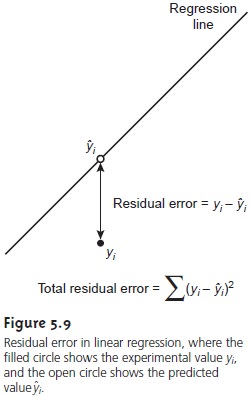
where y is the signal and x is the amount of analyte. The constants β₀ and β₁ are the true y-intercept and the true slope, respectively. The goal of linear regres- sion is to determine the best estimates for the slope, b₁, and y-intercept, b₀. This is accomplished by minimizing the residual error between the experimental val- ues, y_i, and those values, yˆ_i, predicted by equation 5.12 (Figure 5.9). For obvious reasons, a regression analysis is also called a least-squares treatment. Several ap- proaches to the linear regression of equation 5.12 are discussed in the following sections.

Unweighted Linear Regression with Errors in y

The most commonly used form of linear regression is based on three assump- tions: (1) that any difference between the experimental data and the calculated regression line is due to indeterminate errors affecting the values of y, (2) that these indeterminate errors are normally distributed, and (3) that the indetermi- nate errors in y do not depend on the value of x. Because we assume that indeter- minate errors are the same for all standards, each standard contributes equally in estimating the slope and y-intercept. For this reason the result is considered an unweighted linear regression.

The second assumption is generally true because of the central limit theorem. The validity of the two remaining assumptions is less cer- tain and should be evaluated before accepting the results of a linear regression. In particular, the first assumption is always suspect since there will certainly be some indeterminate errors affecting the values of x. In preparing a calibration curve, however, it is not unusual for the relative standard deviation of the mea- sured signal (y) to be significantly larger than that for the concentration of ana- lyte in the standards (x). In such circumstances, the first assumption is usually reasonable.

Finding the Estimated Slope and y-Intercept 

The derivation of equations for cal- culating the estimated slope and y-intercept can be found in standard statistical texts7 and is not developed here. The resulting equation for the slope is given as

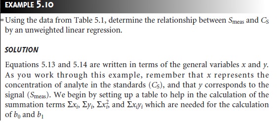
Although equations 5.13 and 5.14 appear formidable, it is only necessary to evaluate four summation terms. In addition, many calculators, spreadsheets, and other com- puter software packages are capable of performing a linear regression analysis based on this model. To save time and to avoid tedious calculations, learn how to use one of these tools. For illustrative purposes, the necessary calculations are shown in de- tail in the following example.

Uncertainty in the Regression Analysis 

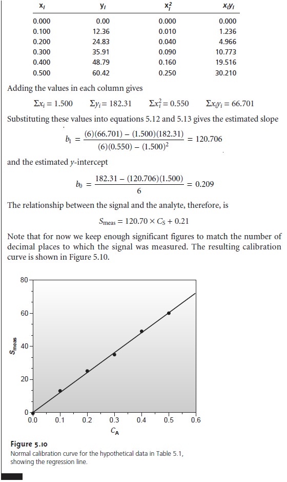
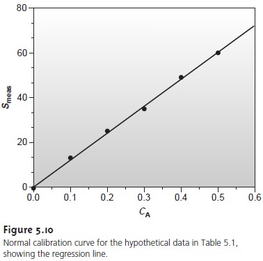
As shown in Figure 5.10, the regression line need not pass through the data points (this is the consequence of indeter- minate errors affecting the signal). The cumulative deviation of the data from the regression line is used to calculate the uncertainty in the regression due to indeterminate error. 

This is called the standard deviation about the regression, s_r, and is given as

There is an obvious similarity between equation 5.15, except that the sum of squares term for s_r is determined rela- tive to yˆ_i instead of yˆ, and the denominator is n – 2 instead of n – 1; n – 2 indicates that the linear regression analysis has only n – 2 degrees of freedom since two pa- rameters, the slope and the intercept, are used to calculate the values of yˆ_i.

A more useful representation of uncertainty is to consider the effect of indeter- minate errors on the predicted slope and intercept. The standard deviation of the slope and intercept are given as

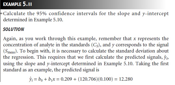
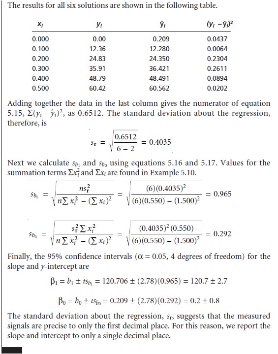
where t is selected for a significance level of α and for n – 2 degrees of freedom. Note that the terms ts_b1 and ts_b0 do not contain a factor of (Root of n )–1 because the con-fidence interval is based on a single regression line. Again, many calculators, spread- sheets, and computer software packages can handle the calculation of s_b0 and s_b1 and the corresponding confidence intervals for β₀ and β_1. Example 5.11 illustrates the calculations.

To minimize the uncertainty in the predicted slope and y-intercept, calibration curves are best prepared by selecting standards that are evenly spaced over a wide range of concentrations or amounts of analyte. The reason for this can be rational- ized by examining equations 5.16 and 5.17. For example, both s_b0 and s_b1 can be minimized by increasing the value of the term Σ(x_i –  x    ‘  )2, which is present in the de-

 nominators of both equations. Thus, increasing the range of concentrations used in preparing standards decreases the uncertainty in the slope and the y-intercept. Fur- thermore, to minimize the uncertainty in the y-intercept, it also is necessary to de- crease the value of the term Σx₁² in equation 5.17. This is accomplished by spreading the calibration standards evenly over their range.

Using the Regression Equation 

Once the regression equation is known, we can use it to determine the concentration of analyte in a sample. When using a normal cali- bration curve with external standards or an internal standards calibration curve, we

 measure an average signal for our sample, Y’_x, and use it to calculate the value of X

where m is the number of replicate samples used to establish Y’_X, n is the number of calibration standards,  yˆ is the average signal for the standards, and x_i and–x’ are the individual and mean concentrations of the standards. Once s_X is known the confi- dence interval for the analyte’s concentration can be calculated as

μ_X= X ± ts_X

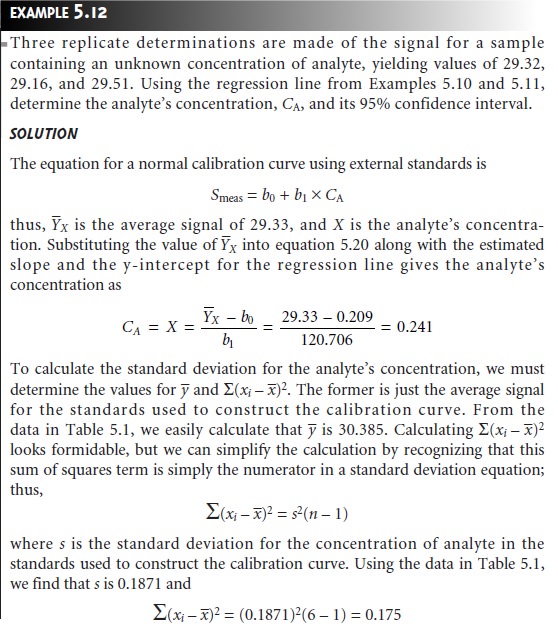
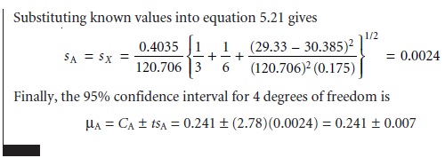
where μ_X is the expected value of X in the absence of determinate errors, and the value of t is determined by the desired level of confidence and for n – 2 degrees of freedom. The following example illustrates the use of these equations for an analysis using a normal calibration curve with external standards.

In a standard addition the analyte’s concentration is determined by extrapolating the calibration curve to find the x-intercept. In this case the value of X is

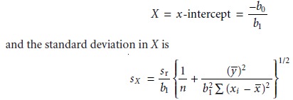
where n is the number of standards used in preparing the standard additions cali- bration curve (including the sample with no added standard), and –y is the average signal for the n standards. Because the analyte’s concentration is determined by ex- trapolation, rather than by interpolation, s_X for the method of standard additions generally is larger than for a normal calibration curve.

A linear regression analysis should not be accepted without evaluating the validity of the model on which the calculations were based. Perhaps the simplest way to evaluate a regression analysis is to calculate and plot the residual error for each value of x. The residual error for a single calibration standard, r_i, is given as

r_i = y_i – yˆ_i

If the regression model is valid, then the residual errors should be randomly distrib- uted about an average residual error of 0, with no apparent trend toward either smaller or larger residual errors (Figure 5.11a). Trends such as those shown in Fig- ures 5.11b and 5.11c provide evidence that at least one of the assumptions on which the regression model is based are incorrect. For example, the trend toward larger residual errors in Figure 5.11b suggests that the indeterminate errors affecting y are not independent of the value of x. In Figure 5.11c the residual errors are not ran- domly distributed, suggesting that the data cannot be modeled with a straight-line relationship. Regression methods for these two cases are discussed in the following sections.

Weighted Linear Regression with Errors in y

Equations 5.13 for the slope, b₁, and 5.14 for the y-intercept, b₀, assume that indeterminate errors equally affect each value of y. When this assumption is false, as shown in Figure 5.11b, the variance associated with each value of y must be included when estimating β₀ and β₁. In this case the predicted slope and intercept are

where w_i is a weighting factor accounting for the variance in measuring y_i. Values of

w_i are calculated using equation 5.24

where s_i is the standard deviation associated with y_i. The use of a weighting factor ensures that the contribution of each pair of xy values to the regression line is proportional to the precision with which y_i is measured.

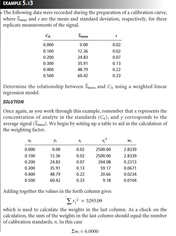
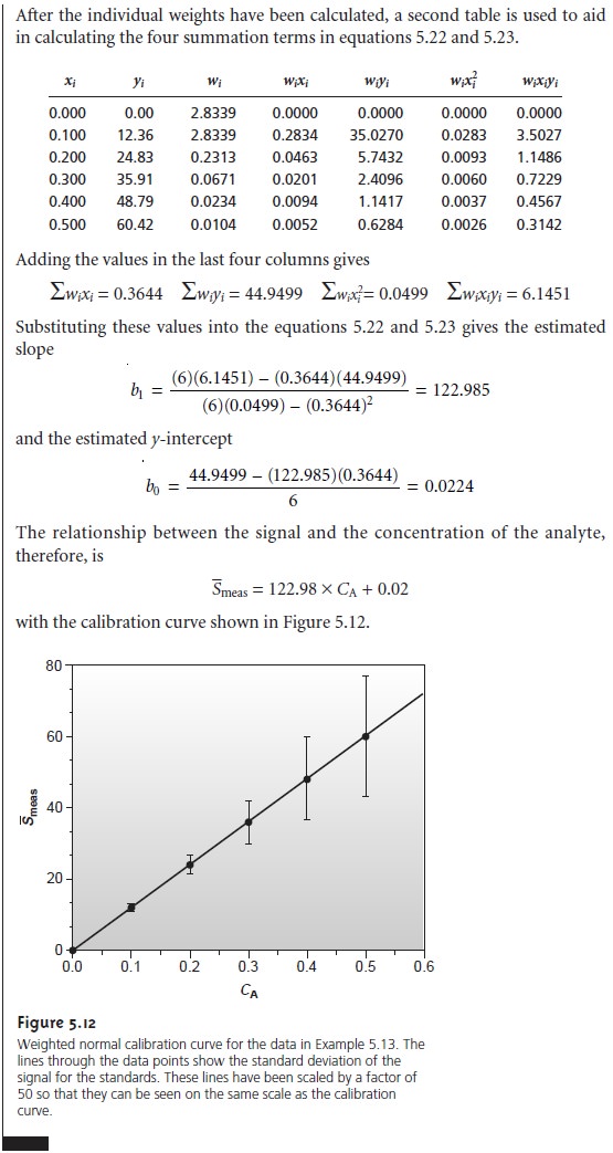
Equations for calculating confidence intervals for the slope, the y-intercept, and the concentration of analyte when using a weighted linear regression are not as easily defined as for an unweighted linear regression. The  confidence in- terval for the concentration of an analyte, however, will be at its optimum valuewhen the analyte’s signal is near the weighted centroid, –y, of the calibration curve

Weighted Linear Regression with Errors in Both x and y

If we remove the assumption that the indeterminate errors affecting a calibration curve are found only in the signal (y), then indeterminate errors affecting the preparation of standards containing known amounts of analyte (x) must be fac- tored into the regression model. The solution for the resulting regression line is computationally more involved than that for either the unweighted or weighted regression lines, and is not presented in this text.

Curvilinear and Multivariate Regression

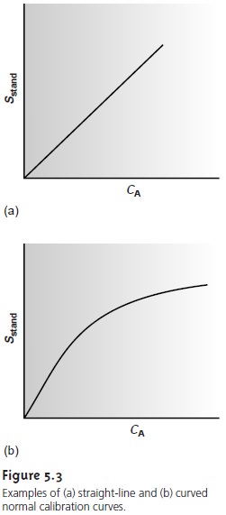
Regression models based on a straight line, despite their apparent complexity, use the simplest functional relationship between two variables. In many cases, calibra- tion curves show a pronounced curvature at high concentrations of analyte (see Figure 5.3b). One approach to constructing a calibration curve when curvature exists is to seek a transformation function that will make the data linear. Logarithms, expo- nentials, reciprocals, square roots, and trigonometric functions have all been used in this capacity. A plot of y versus log x is a typical example. Such transformations are not without complications. Perhaps the most obvious is that data that originally has a uniform variance for the y values will not maintain that uniform variance when the variable is transformed.

A more rigorous approach to developing a regression model for a nonlinear calibration curve is to fit a polynomial equation such as y = a + bx + cx2 to the data. Equations for calculating the parameters a, b, and c are derived in the same manner as that described earlier for the straight-line model. When a single polynomial equation cannot be fitted to the calibration data, it may be possible to fit separate polynomial equations to short segments of the calibration curve. The result is a sin- gle continuous calibration curve known as a spline function.

The regression models considered earlier apply only to functions containing a single independent variable. Analytical methods, however, are frequently subject to determinate sources of error due to interferents that contribute to the measured sig- nal. In the presence of a single interferent, equations 5.1 and 5.2 become

S_meas = k_An_A + k_In_I + S_reag

S_meas = k_AC_A + k_IC_I + S_reag

where k_I is the interferent’s sensitivity, n_I is the moles of interferent, and C_I is the in- terferent’s concentration. Multivariate calibration curves can be prepared using standards that contain known amounts of analyte and interferent.