Least Cost Input

LEAST COST INPUT:

1. Optimal Input Level

Given the marginal revenue product and marginal factor cost, one can compute the optimal amount of the variable input for using it in the production process.

An economic activity should be expanded as long as the marginal benefits exceed the marginal costs. The optimal point occurs at the point where the marginal benefits are equal to the marginal costs. MRPx = MFCx

2. Single Input System

Profit maximization requires production at a level where the marginal revenue is equal to the marginal cost. Because the only variable in the system is input L, the marginal cost of production is as follows:

MC =       TC/       Output

MC =PL/MPL

Since marginal revenue should be equal to the marginal cost at the profit-maximizing level,

A profit-maximizing firm always employs an input upto the point where its marginal revenue product equals its cost.

1. The firm can employ as much labor as it needs by paying workers $50 per period (the labor market is considered perfectly competitive).

2. The firm can sell all the ore it can produce at a price of $10 per ton MRP = MFC = $50

3. In a case of less than six workers, MRP > MFC and the addition of more workers will increase revenue. Beyond six, the opposite is true.

The Production Function with Two Variable Inputs

In the ore-mining example, assume that both capital and labor are now variable.

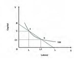
1. Production Isoquant

A production isoquant is either a geometric curve or an algebraic function representing all the various combinations of the two inputs that can be used in producing a given level of output. It can also be defined as a curve (a locus of points) showing all possible combinations of inputs physically capable of producing a given fixed level of output.

2. Marginal Rate of Technical Substitution

It is the rate at which one input may be substituted for another input in the production process. It can also be defined as the rate at which one input is substituted for another along an isoquant. The rate of change of one variable with respect to another variable is given by the slope of a curve relating the two variables. Thus, the rate of change of input Y with respect to X, i.e. the rate at which Y may be substituted for X in the production process is given by the slope of the curve relating Y to X. This is the slope of the isoquant.

Since the slope is negative and one wishes to express the substitution rate as a positive quantity, a negative sign is attached to the slope.

MRTS =Y1 - Y2/X1 - X2=   Y/  X

OQUANT

In economics, an isoquant (derived from quantity and the Greek word iso, meaning equal) is a contour line drawn through the set of points at which the same quantity of output is produced while changing the quantities of two or more inputs. While an indifference curve mapping helps to solve the utility-maximizing problem of consumers, the isoquant mapping deals with the cost-minimization problem of producers. Isoquants are typically drawn on capital-labor graphs, showing the technological tradeoff between capital and labor in the production function, and the decreasing marginal returns of both inputs. Adding one input while holding the other constant eventually leads to decreasing marginal output, and this is reflected in the shape of the isoquant. A family of isoquants can be represented by an isoquant map, a graph combining a number of isoquants, each representing a different quantity of output. Isoquants are also called equal product curves.

An isoquant shows the extent to which the firm in question has the ability to substitute between the two different inputs at will in order to produce the same level of output. An isoquant map can also indicate decreasing or increasing returns to scale based on increasing or decreasing distances between the isoquant pairs of fixed output increment, as you increase output. If the distance between those isoquants increases as output increases, the firm's production function is exhibiting decreasing returns to scale; doubling both inputs will result in placement on an isoquant with less than double the output of the previous isoquant. Conversely, if the distance is decreasing as output increases, the firm is experiencing increasing returns to scale; doubling both inputs results in placement on an isoquant with more than twice the output of the original isoquant.

As with indifference curves, two isoquants can never cross. Also, every possible combination of inputs is on an isoquant. Finally, any combination of inputs above or to the right of an isoquant results in more output than any point on the isoquant. Although the marginal product of an input decreases as you increase the quantity of the input while holding all other inputs constant, the marginal product is never negative in the empirically observed range since a rational firm would never increase an input to decrease output.