Indifference Curve Approach : Definition, Schedule, curve, map

Indifference Curve Approach

Marshall's demand analysis is based on the cardinal measurement of utility. The approach is criticised for two reasons.

1.        Utility is a psychological phenomenon and

2.        It cannot be measured.

Hence, the indifference curve approach based on ordinal ranking preference was evolved. Vilfred Pareto, Wicksteed and Slutsky developed this approach. Two noted English economists Prof. J.R. Hicks and Prof. Allen provided a refined version of indifference curve approach. According to Hicks and Allen, utility cannot be measured. It can only be ranked or ordered. The consumer can rank his preference very easily and say which is better than the other.

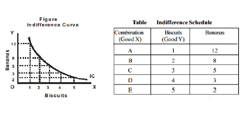
The concept of scale of preference has been explained by indifference curve. An indifference curve shows different combinations of two commodities, which give the consumer an equal satisfaction.

Definition

An indifference curve is the locus of different combinations of two commodities giving the same level of satisfaction.

Assumptions of indifference curve analysis

1.        The consumer is rational. So, he prefers more goods to less goods.

2.        He purchases two goods, X and Y only.

3.        The price that a consumer pays for a commodity indicates the level of utility derived by him.

4.        His income remains constant

5.        His tastes, preferences, habits remain unchanged.

Indifference Schedule

An indifference schedule is a statement of various combinations of two commodities that will equally be accepted by the consumer. The various combinations give equal satisfaction to the consumer. Therefore he is indifferent between various combinations.

Let us assume that the consumer buys two commodities - bananas and biscuits. Then the indifference schedule will be:

Indifference Schedule

          Combination       Biscuits       Bananas

          (Good X)    (Good Y)            

          A       1        12     

          B       2        8       

          C       3        5       

          D       4        3       

          E       5        2

From the above schedule it can be understood that while the number of biscuits is increasing, the number of bananas is decreasing so that the level of satisfaction is the same for all the combinations. Therefore the consumer is indifferent between the combinations A, B, C, D and E.

Indifference curve

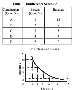
The data in the indifference schedule can be represented in the graph with one commodity on the X-axis and another commodity in the Y-axis The various combinations of the two commodities are plotted and joined to form a curve called indifference curve. In the figure IC is an indifference curve showing combinations of the two commodities given in the schedule.

All the points on this curve give equal level of satisfaction to the consumer. Indifference curve is otherwise called 'iso -utility curve'.

Indifference Map

Indifference Map is a group of indifference curves for two commodities showing different levels of satisfaction. In this indifference map, it should be clearly understood that a higher indifference curve denotes higher level of satisfaction and a lower indifference curve represents lower level of satisfaction. Being rational, the consumer will always choose a higher indifference curve to get maximum satisfaction, other things being equal.

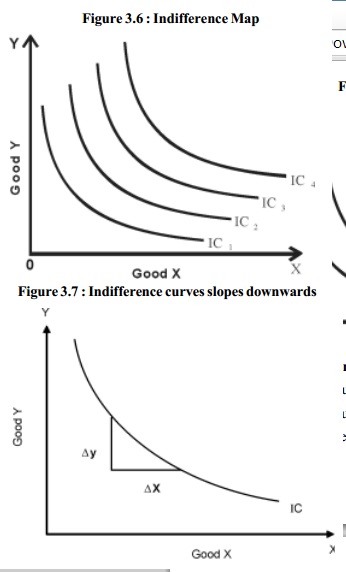
Properties of an Indifference curve

1.        Indifference curves slope downwards to the right

2.        Indifference curves are convex to the origin

No two indifference curves can ever cut each other.

All indifference curves slope downwards from left to right

The downward slope of indifference curve must be attributed to the fact that the consumer in substituting good X by good Y, increases the amount of Y and reduces the amount of X. If the indifference curve were horizontal line running parallel to X axis then the combination which it represents is the same amount of Y but more and more of X. In that case, the satisfaction from the combination will not be equal. For the same reason, it can be said that indifference curve will not be vertical.

All indifference curves are convex to the origin

This is because of the operation of a principle known as 'Diminishing Marginal Rate of Substitution'. The indifference curves are based on this principle. If they are concave to the origin, then it will mean that MRS is increasing. Indifference curve cannot be straight line except when the goods are perfect substitutes.

Marginal rate of substitution between X and Y referes to the amount of commodity Y to be offered in exchange for one unit of X commodity. The MRS goes on diminishing as consumer goes on substituting X for Y.

The third assumption is that no two indifference curves can ever cut each other. But in Figure 3.8 we find two indifference curves do cut each other.

Point A which is on indifference curve 2 represents a higher level of satisfaction to the consumer than at point B which is on indifference curve 1. But point C lies on both curves. That means, two levels of satisfaction A and B which are unequal have become equal. That cannot be accepted. So indifference curves can never cut each other.

These are the three assumptions about the shape of an indifference curve.

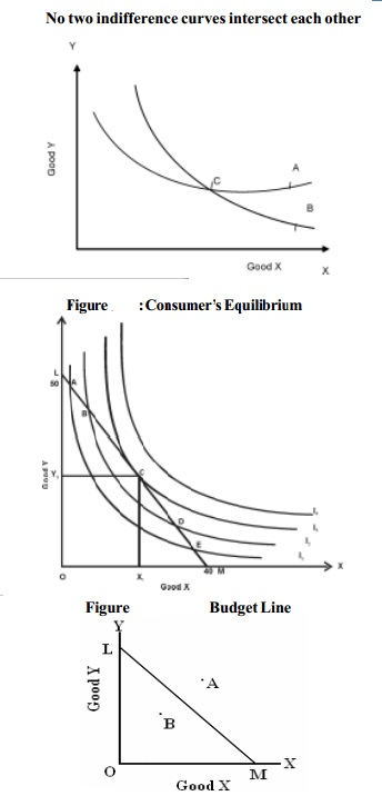
Consumer's Equilibrium through Indifference Curve Analysis

As a consumer has a limited income, he spends it in such a manner so as to obtain maximum level of satisfaction. He will attain equilibrium when he gets maximum satisfaction from his expenditure on different goods. Under the utility analysis explained earlier, a consumer gets maximum satisfaction when marginal utilities from his different purchases are equal. We can also explain the equilibrium of the consumer with the help of the indifference curve analysis. For our analysis, we have to make the following assumptions.

1.        The consumer has before him an indifference map for a pair of goods say, tea and biscuits. This map represents the preferences of the consumer for the two goods. It is assumed that his scales of preferences remain constant at a given time.

2.        The consumer has a fixed amount of money to spend on the two goods. It is assumed that he will spend the amount on both the goods and not save any part of it.

3.        The prices of these goods are given in the market and are assumed to be constant.

4.        The consumer is assumed to act rationally and maximise his satisfaction.

A consumer's indifference map for good X and good Y is given in figure 3.6; it represents four scales of preferences of a consumer for the two goods. Indifference curves to the right represent higher satisfaction. The consumer would like to choose a combination of good X and good Y, which will be on the highest indifference curve. But his choice will depend upon his income and the price of the two goods.

To understand the extent of purchase of the goods with the given prices and income of the consumer, budget line is important.

Budget line of the consumer

Suppose that the consumer has Rs.20 to spend on tea and biscuits, which cost 50 paise and 40 paise respectively. The consumer has three alternative possibilities before him.

1.        He may decide to buy tea only, in which case he can buy 40 cups of tea.

2.        He may decide to buy biscuits only, in which case he can buy 50 biscuits.

3.        He may decide to buy some quantity of both the goods, say 20 cups of tea (Rs.10) and 25 biscuits (Rs.10) or 12 cups of tea (Rs.6) and 35 biscuits (Rs.14), and so on. (Total amount = Rs.20).

Figure  shows the above three possibilities. The line LM represents maximum amount of biscuits (50) and to tea (40 cups), which the consumer can buy with his income of Rs.20. The line LM shows that the consumer cannot choose any combination beyond this line because his income does not permit him. Nor would he like to choose a combination below this line; say, B, as it will not represent the maximum satisfaction.

Line LM is known as the budget line since it represents the various amounts the consumer can buy with his income; it is also known as the price-ratio line or simply the price line since its slope represents the ratio of prices of the two goods (i.e., OM of Good X = OL of good Y).

The consumer gets the maximum possible satisfaction from his given income at point C on the indifference curve I3. At this point, he buys a combination of OX1 amount of Good X and OY1 amount of Good Y. Any other possible combination of the two goods will either yield lesser satisfaction or will not be unobtainable at present prices, with the given amount of income of the consumer.

At the point of equilibrium (point C) the price-line LM is tangential to the indifference curve I3. At point C, the indifference curve and the price-line have the same slope. Now the slope of the indifference curve represents the marginal rate of substitution; and the budget line shows the ratio of prices between the two goods. At point C the marginal rate substitution between the two goods as indicated by the slope of the indifference curve I3 and the ratio of prices between the two goods as indicated by the price-line LM are equal. This point, therefore, indicates the ideal combination between the two commodities, giving the consumer the highest satisfaction possible with his limited income. At this point, therefore the consumer is in equilibrium.

The fundamental condition of equilibrium is that the marginal rate of substitution of commodity X for commodity Y should be equal to the ratio of prices between the two goods. Therefore, the condition for equilibrium is MRSxy = Px / Py