Dijkstra’s Algorithm

Dijkstra’s Algorithm

In this section, we consider the single-source shortest-paths problem: for a given vertex called the source in a weighted connected graph, find shortest paths to all its other vertices. It is important to stress that we are not interested here in a single shortest path that starts at the source and visits all the other vertices. This would have been a much more difficult problem (actually, a version of the traveling salesman problem introduced in Section 3.4 and discussed again later in the book). The single-source shortest-paths problem asks for a family of paths, each leading from the source to a different vertex in the graph, though some paths may, of course, have edges in common.

A variety of practical applications of the shortest-paths problem have made the problem a very popular object of study. The obvious but probably most widely used applications are transportation planning and packet routing in communi-cation networks, including the Internet. Multitudes of less obvious applications include finding shortest paths in social networks, speech recognition, document formatting, robotics, compilers, and airline crew scheduling. In the world of enter-tainment, one can mention pathfinding in video games and finding best solutions to puzzles using their state-space graphs (see Section 6.6 for a very simple example of the latter).

There are several well-known algorithms for finding shortest paths, including Floyd’s algorithm for the more general all-pairs shortest-paths problem discussed in Chapter 8. Here, we consider the best-known algorithm for the single-source shortest-paths problem, called Dijkstra’s algorithm.⁴ This algorithm is applicable to undirected and directed graphs with nonnegative weights only. Since in most ap-plications this condition is satisfied, the limitation has not impaired the popularity of Dijkstra’s algorithm.

Dijkstra’s algorithm finds the shortest paths to a graph’s vertices in order of their distance from a given source. First, it finds the shortest path from the source

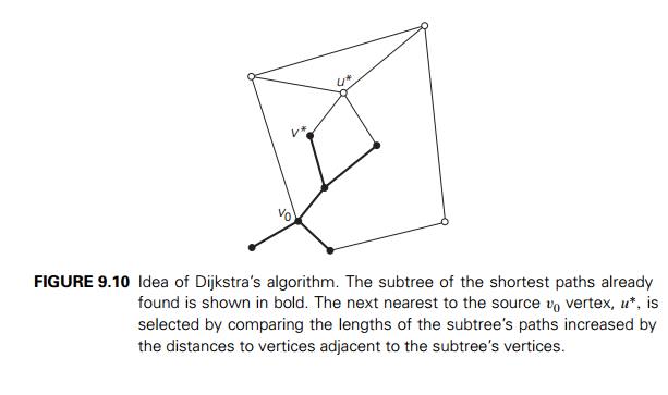
to a vertex nearest to it, then to a second nearest, and so on. In general, before its ith iteration commences, the algorithm has already identified the shortest paths to i − 1 other vertices nearest to the source. These vertices, the source, and the edges of the shortest paths leading to them from the source form a subtree T_i of the given graph (Figure 9.10). Since all the edge weights are nonnegative, the next vertex nearest to the source can be found among the vertices adjacent to the vertices of T_i. The set of vertices adjacent to the vertices in T_i can be referred to as “fringe vertices”; they are the candidates from which Dijkstra’s algorithm selects the next vertex nearest to the source. (Actually, all the other vertices can be treated as fringe vertices connected to tree vertices by edges of infinitely large weights.) To identify the ith nearest vertex, the algorithm computes, for every fringe vertex u, the sum of the distance to the nearest tree vertex v (given by the weight of the edge (v, u)) and the length d_v of the shortest path from the source to v (previously determined by the algorithm) and then selects the vertex with the smallest such sum. The fact that it suffices to compare the lengths of such special paths is the central insight of Dijkstra’s algorithm.

To facilitate the algorithm’s operations, we label each vertex with two labels. The numeric label d indicates the length of the shortest path from the source to this vertex found by the algorithm so far; when a vertex is added to the tree, d indicates the length of the shortest path from the source to that vertex. The other label indicates the name of the next-to-last vertex on such a path, i.e., the parent of the vertex in the tree being constructed. (It can be left unspecified for the source s and vertices that are adjacent to none of the current tree vertices.) With such labeling, finding the next nearest vertex u^∗ becomes a simple task of finding a fringe vertex with the smallest d value. Ties can be broken arbitrarily.

After we have identified a vertex u^∗ to be added to the tree, we need to perform two operations:

Move u^∗ from the fringe to the set of tree vertices.

For each remaining fringe vertex u that is connected to u^∗ by an edge of weight w(u^∗, u) such that d_u∗ + w(u^∗, u) < d_u, update the labels of u by u^∗ and d_u∗ + w(u^∗, u), respectively.

Figure 9.11 demonstrates the application of Dijkstra’s algorithm to a specific graph.

The labeling and mechanics of Dijkstra’s algorithm are quite similar to those used by Prim’s algorithm (see Section 9.1). Both of them construct an expanding subtree of vertices by selecting the next vertex from the priority queue of the remaining vertices. It is important not to mix them up, however. They solve different problems and therefore operate with priorities computed in a different manner: Dijkstra’s algorithm compares path lengths and therefore must add edge weights, while Prim’s algorithm compares the edge weights as given.

Now we can give pseudocode of Dijkstra’s algorithm. It is spelled out— in more detail than Prim’s algorithm was in Section 9.1—in terms of explicit operations on two sets of labeled vertices: the set V_T of vertices for which a shortest path has already been found and the priority queue Q of the fringe vertices. (Note that in the following pseudocode, V_T contains a given source vertex and the fringe contains the vertices adjacent to it after iteration 0 is completed.)

ALGORITHM     Dijkstra(G, s)

//Dijkstra’s algorithm for single-source shortest paths

//Input: A weighted connected graph G =  V , E  with nonnegative weights

            and its vertex s

//Output: The length d_v of a shortest path from s to v

// and its penultimate vertex p_v for every vertex v in V Initialize(Q) //initialize priority queue to empty

for every vertex v in V

d_v ← ∞;        p_v ← null

Insert(Q, v, d_v) //initialize vertex priority in the priority queue d_s ← 0; Decrease(Q, s, d_s) //update priority of s with d_s

V_T ← ∅

for i ← 0 to |V | − 1 do

u^∗ ← DeleteMin(Q)          //delete the minimum priority element

V_T ← V_T ∪ {u^∗}

for every vertex u in V − V_T that is adjacent to u^∗ do if d_u∗ + w(u^∗, u) < d_u

d_u ← d_u∗ + w(u^∗, u);           p_u ← u^∗

Decrease(Q, u, d_u)

The time efficiency of Dijkstra’s algorithm depends on the data structures used for implementing the priority queue and for representing an input graph itself. For the reasons explained in the analysis of Prim’s algorithm in Section 9.1, it is

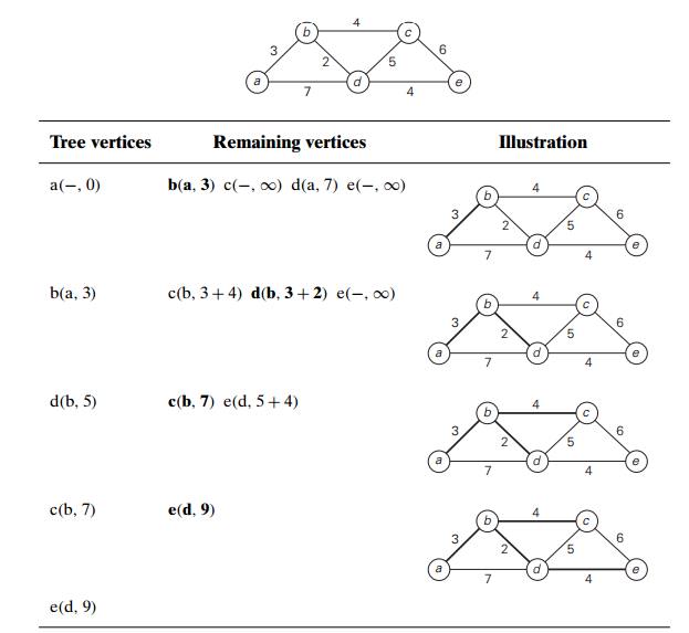
The shortest paths (identified by following nonnumeric labels backward from a destination vertex in the left column to the source) and their lengths (given by numeric labels of the tree vertices) are as follows:

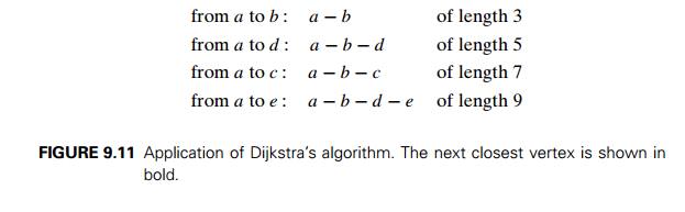
FIGURE 9.11 Application of Dijkstra’s algorithm. The next closest vertex is shown in bold.

in  $(|V |²) for graphs represented by their weight matrix and the priority queue implemented as an unordered array. For graphs represented by their adjacency lists and the priority queue implemented as a min-heap, it is in O(|E| log |V |). A still better upper bound can be achieved for both Prim’s and Dijkstra’s algorithms if the priority queue is implemented using a sophisticated data structure called the Fibonacci heap (e.g., [Cor09]). However, its complexity and a considerable overhead make such an improvement primarily of theoretical value.

Exercises 9.3

            Explain what adjustments if any need to be made in Dijkstra’s algorithm and/or in an underlying graph to solve the following problems.

            Solve the single-source shortest-paths problem for directed weighted graphs.

            Find a shortest path between two given vertices of a weighted graph or digraph. (This variation is called the single-pair shortest-path problem.)

            Find the shortest paths to a given vertex from each other vertex of a weighted graph or digraph. (This variation is called the single-destination shortest-paths problem.)

            Solve the single-source shortest-paths problem in a graph with nonnegative numbers assigned to its vertices (and the length of a path defined as the sum of the vertex numbers on the path).

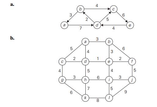
Solve the following instances of the single-source shortest-paths problem with vertex a as the source:

            Give a counterexample that shows that Dijkstra’s algorithm may not work for a weighted connected graph with negative weights.

            Let T be a tree constructed by Dijkstra’s algorithm in the process of solving the single-source shortest-paths problem for a weighted connected graph G.

                                                                            True or false: T is a spanning tree of G?

                                                                            True or false: T is a minimum spanning tree of G?

            Write pseudocode for a simpler version of Dijkstra’s algorithm that finds only the distances (i.e., the lengths of shortest paths but not shortest paths themselves) from a given vertex to all other vertices of a graph represented by its weight matrix.

            Prove the correctness of Dijkstra’s algorithm for graphs with positive weights.

            Design a linear-time algorithm for solving the single-source shortest-paths problem for dags (directed acyclic graphs) represented by their adjacency lists.

            Explain how the minimum-sum descent problem (Problem 8 in Exercises 8.1) can be solved by Dijkstra’s algorithm.

            Shortest-path modeling Assume you have a model of a weighted connected graph made of balls (representing the vertices) connected by strings of appro-priate lengths (representing the edges).

                                                                            Describe how you can solve the single-pair shortest-path problem with this model.

                                                                            Describe how you can solve the single-source shortest-paths problem with this model.

            Revisit the exercise from Section 1.3 about determining the best route for a subway passenger to take from one designated station to another in a well-developed subway system like those in Washington, DC, or London, UK. Write a program for this task.