Continuous Versus Discrete Control

CONTINUOUS VERSUS DISCRETE CONTROL

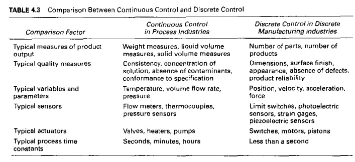
Industrial control systems used in the process industries have tended to emphasize the control of continuous variables and parameters. By contrast, the manufacturing industries produce discrete parts and products, and the controllers used here have tended to emphasize discrete variables and parameters. Just as we have two basic types of variables and parameters that characterize production operations, we also have two basic types of control:

(1) continuous control, in which the variables and parameters are continuous and analog; and (2) discrete control, in which the variables and parameters are discrete, mostly binary discrete. Some of the differences between continuous control and discrete control are summarized in Table 4.3.

In reality, most operations in the process and discrete manufacturing industries tend to include both continuous as well as discrete variables and parameters. Consequently, many industrial controllers are designed with the capability to receive, operate on, and transmit both types of signals and data. In Chapter 5, we discuss the various types of sig

nals and data in industrial control systems and how the data are converted for use by dig" ital computer controllers.

       To complicate mailers, with the substitution of the digital computer to replace analog controllers in continuous process control applications starting around 1960 (Historical Note 4.1), continuous process variables are no longer measured continuously. Instead, they are sampled periodically, in effect creating a discrete sampleddata system that approximates the actual coruinuous system. Similarly, the control signals sent to the process are typically stepwise functions that approximate the previous continuous control signals transmitted by analog controllers. Hence, in digital computer process control, even continuous van abies and parameters possess characteristics of discrete data, and these characteristics must be considered in the design of the computer process interface and the control algorithms used by the controller

       Continuous Control Systems

In continuous control, the usual objective is to maintain the value of an output variable et a desired level, similar to the operation of a feedback control system as defined in the previous chapter (Section 3.1.3). However, most continuous processes in the practical world consist of many separate feedback loops, all of which have to be controlled and coordinated to maintain the output variable at the desired value. Examples of continuous processes are the following:

   Control of the uuiput of a chemical reaction that depends on temperature, pressure, lind input flow rates of several reactants. All of these variables and/or parameters are continuous .

   Control of the position of a workpart relative to a cutting tool in a contour milling operation in which complex curved surfaces are generated. The position of the part is defined by X, j'. and acoordinate values. As the part moves, the x, y, and z values can he considered as continuous variables and/or parameters that change over lime to machine the part.

There      are several  approaches   by which the control      objective     is achieved  in a continuous process control system.In the following paragraphs, we survey the most prominent categories,

       Regulatory Control. In regulatory control, the objective is to maintain process performance at a certain level or within a given tolerance band of that level. This is appropriate, for example, when the performance attribute is some measure of product quality, and it is

important to keep the quality at the specified level Of within a specified range. In many applications, the performance measure of the process, sometimes called the index of performance. must be calculated based on several output variables of the process. Except for this feature. regulatory control is to the overall process what feedback control is 10 an individual control loop in the process, as suggested hy Figure 4.2

The trouble with regulatory control (the same problem exists with a simple feedback control loop) is that compensating action is taken only after a disturbance has affected the process output. An error must be present for any control action to be taken. The presence of an error means that the output of the process is different from the desired value. The following control mode, fcedforwanl control, addresses this issue.

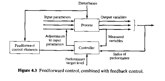
       Feedforward Control. The strategy in feedforward control is to anticipate the effeet of disturbances that will upset the process by sensing them and compensating for them before they can affect the process. As shown in Figure 4.3, the Ieedforward control elements sense the presence of a disturbance and take corrective action by adjusting a process parameter that compensates for any effect the disturbance will have on the process. In the ideal case, the compensation is completely effective. However, complete compensation is unlikely because of imperfections in the feedback measurements, actuator operations, and control algorithms, so feedforward control is usually combined with feedback control, as shown in our figure. Regulatory and feedforward control are more closely associated with the process industries than with discrete product manufacturing

Steady State Optimization. This term refers to a class of optimization techniques in which the process exhibits the followingchaHleteristics: (1) there is a welldefined index of performance, such as product cost, production rate, or process yield; (2) the relationship between the process variables and the index of performance is known; and (3) the values of the system parameters that optimize the index of performance can be determined mathematically. When these characteristics apply, the control algorithm is designed to make adjustments in the process parameters to drive the process toward the optimal state. The control system is openloop, as seen in Figure 4.4, Several mathematical techniques are available for solving steadystate optimal control problems, including differential calculus, calculus of variations, and a variety of mathematical programming methods.

Adaptive Control. Steadystate optimal control operates as an openloop system It works successfullv when there are no disturbances that invalidate the known relationship between process parameters and process performance. When such disturbances are present in the application, a selfcorrecting form of optimal control can be used, called adaptive control. Adaptive controlcombines feedback control and optimal control by measuring the relevant process variables during operation (as in feedback control) and using a control algorithm that attempts to optimize some index of performance (as in optimal control).

Adaptive control is distinguished from feedback control and steadystate optimal cuntrol by its unique capability to cope with a timevarying environment. It is not unusual for a system to operate in an environment thai changes over time and for the changes to have a potential effect on system performance. If the internal parameters or mechanisms of the system are fixed, as in feedback control or optimal control, the system may perform quite differently in one type of environment than in another. An adaptive control system is designed to compensate for its changing environment by monitoring its own performance and altering some aspect of its control mechanism to achieve optimal or nearoptimal performance. In a production process, the "timevarying environment" consists of the daytoday variations in raw materials, tooling, atmospheric conditions, and the like, any of which may affect performance

The general configuration of an adaptive control system is illustrated in Figure 4.5To evaluate its performance and respond accordingly, an adaptive control system performs three functions, as shown in the figure:

       Identification function. In this function, the current value of the index of performance of the system is determined, based on measurements collected from tbe process. Since

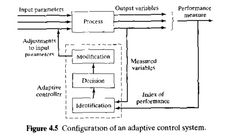
the environment changes over time, system performance also changes. Accordingly, the identification function must be accomplished more or less continuously over time during system operation

    Decision function. Once system performance has been determined, the next function is to decide what changes should be made to improve performance. The decision function is implemented by means of the adaptive system's programmed algorithm. Depending on this algorithm. the decision may be to change one or more input parameters to the process, to alter some of the internal parameters of the controller, or other changes

3, Modification function, The third function of adaptive control is to implement the decision. Whereas decision is a logic function, modification is concerned with physical changes in thc system. It involves hardware rather than software. In modification, the system parameters or process inputs are altered using available actuators to drive the system toward a more optimal state,

Adaptive control is most applicable at levels Land 3 in our automation hierarchy (Table 4.2).Adaptive control has been the subject of research and development for several decades, originally motivated by problems of highspeed flight control in the age of jet aircraft. The principles have been applied in other areas as well,inc1udingmanufacturing.

One  notable        effort is adaptive  control        machining.

       OnLine Search Strategies. Online search strategies can be used to address a special class of adaptive control problem in which the decision function cannot be sufficiently defined: that is, the relationship between the input parameters and the index of performance is not known, or nor known well enough to use adaptive control as previously described. Therefore, it is not possible to decide on the changes in the internal parameters of the system to produce the desired performance improvement. Instead, experiments must be performed all the process. Small systematic changes are made in the input parameters of the process to observe what effect these changes will have on the output variables. Based on the results of these experiments, larger changes are made in the input parameters to drive the process toward improved performance.

Online search strategies include a variety of schemes to explore the effects of changes in process parameters, ranging from trialanderror techniques to gradient methods. All of the schemes attempt to determine which input parameters cause the greatest positive effect on the index of performance and then move tile process in that direction. There is little evidence that online search techniques are used much in discrete parts manufacturing.

Their applications   are more  common      in the continuous  process       industries.

Other Specialized Techniques. Other specialized techniques include strategies that are currently evolving in control theory and computer science. Examples include learning systems, expert systems, neural networks, and other artificial intelligence methods for process control

       Discrete Control  Systems

In discrete control, the parameters and variables of the system are changed at discrete moments in time. The changes involve variables and parameters that are also discrete, typically binary (ON/OFF). The changes are defined in advance by means of a program of instructions, for example, a work cycle program (Section 3.1.2). The changes are executed either because the state of the system has changed or because a certain amount of time has elapsed. These two cases can be distinguished as (1) eventdriven changes or (2) timedriven changes [3J

An eventdriven change is executed by the controller in response to some event that has caused the state of the system to he altered. The change can be to initiate an operation or terminate an operation, start a motor or stop it, open a valve or close it, and so forth. Examples of eventdriven changes are'

   A robot loads a workparl into the fixture, and the part is sensed by a limit switch. Sensing the part's presence is the event that alters the system state. The eventdriven change is that the automatic machining cycle can now commence.

   The diminishing level of plastic molding compound in the hopper of an injection molding machine triggers a lowlevel switch, which in tum triggers a valve to open that starts the flow of new plastic into the hopper. When the level of plastic reaches the highlevel switch, this triggers the valve to close, thus stopping the flow of pellets into the hopper

   Counting parts moving along a conveyor past an optical sensor is an eventdriven system. Each part moving past the sensor is an event that drives the counter.

A timedriven change is executed by the control system either at a specific point in time or after a certain time lapse has occurred. As before, the change usually consists of starting something or stopping something, and the time when the change occurs is important. Examples of timedriven changes are:

   In factories with specific starting times and ending times for the shift and uniform break periods for all workers, the "shop clock" is set to sound a bell at specific moments during the day to indicate these start and stop times.

Heat treating operations must be carried out for a certain length of time. An automated heat treating cycle consists of automatic loading of parts into the furnace (perhaps by a robot) and then unloading after the parts have been heated for the specified length of time.

   In the operation of a washing machine, once the laundry tub has been filled to the preset level, the agitation cycle continues for a length of time set on the controls. When this tune is up, the timer stops the agitation and initiates draining of the tub. (By comparison with the agitation cycle. filling the laundry tub with water is eventdriven. Filling continues until the proper level has been sensed, which causes the inlet valve to close.)

The two types of change correspond to two different types of discrete control, called combinational logic control and sequertual control. Combinational logic control is used to control the execution of eventdriven changes, and sequential control is used to manage timedriven changes. These types of control are discussed in our expanded coverage of discrete control in ChapterS

Discrete control is widely used in discrete manufacturing as well as the process in dustries. In discrete manufacturing, it is used to control the operation of conveyors and other material transport systems (Chapter 10), automated storage systems (Chapter 11) standalone production machines (Chapter 14), flexible manufacturing systems (Chapter 16),automated transfer lines (Chapter lS),and automated assembly systems (Chapter 19). All of these systems operate by following a welldefined sequence of startandstop actions, such as powered feed motions, parts transfers between workstations, and online automated inspections, which are wellsuited to discrete control.

In the process industries, discrete control is associated more with batch processing than with continuous processes. In a typical batch processing operation, each batch of starting ingredients is subjected to a cycle of processing steps that involves changes in process parameters (e.g., temperature and pressure changes),possible flow from one container to another during the cycle, and finally packaging. The packaging step differs depending on the product. For foods, packaging may involve canning or boxing. For chemicals, it means filling containers with the liquid product. And for pharmaceuticals, it may involve filling bottles with medicine tablets. In batch process control, the objective is to manage the sequence and timing of processing steps as well as to regulate the process parameters in each step. Accordingly, batch process control typically includes both continuous control as well as discrete control.