Chapter: 11th Computer Technology : Chapter 11 : Data Tools and Printing
Applying conditional format - OpenOffice Calc
Applying
conditional format
Important
aspect of the data tools lies in the visualization of those data for easy
understanding of the user. Conditional formatting gives different font size,
font colour and background colour for different data, based on the user
requirements.
You
can set up cell formats to change font size, font colour, background colour
depending on conditions that you specify. For example, in a table of numbers,
you can show all the values above the average in green and all those below the
average in red.
For
example, the marks of the students are entered in the spreadsheet. The marks
should be shown in different colours for the different marks ranges.
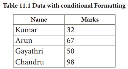
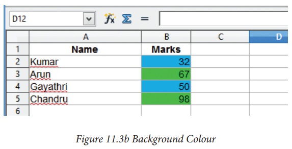
Illustration 11.1: Apply the conditional formatting for Table 11.1 as for the condition given below.
1.
Marks less than or equal to 50 in Lightgreen
2.
Marks greather than 50 in blue
Table 11.1 Data with conditional Formatting
![]()
![]()
![]()
![]()
![]()
Procedure to apply conditional formatting:
1.
Select the cells which contain marks
2.
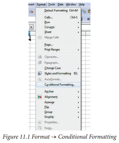
Choose Format → Conditional Formatting from the menu bar
3.
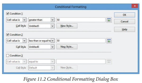
Conditional formatting dialog box appears as shown in Figure 11.2
4.
Select Condition 1, choose cell value
is “greater than” and type 50 in the
value box.
5.
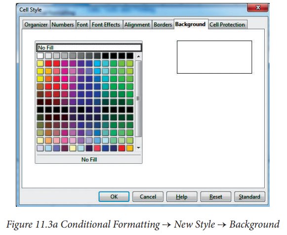
Then click New Style button. The New
Style button has various options such as Font Style, Font Size, Font colour,
Font alignment, Border Colour, and Background colour.
Now,
the cell style dialog box appears as shown in Figure 11.3a will appear. Click
Background Tab and choose light green.
6.
Similarly, Select Condition 2, choose cell value is “less than” and type 50 in
the value box. In the background tab, choose blue colour.
Finally
OpenOffice calc shows the result as given
below:
Related Topics