Chapter: Civil : Construction Planning And Scheduling : Quality Control and Safety during Construction
Statistical Quality Control with Sampling by Variables

Statistical
Quality Control with Sampling by Variables
As described in the previous section, sampling by
attributes is based on a classification of items as good or defective. Many work
and material attributes possess continuous properties, such as strength,
density or length. With the sampling by attributes procedure, a particular
level of a variable quantity must be defined as acceptable quality. More
generally, two items classified as good might have quite different strengths or
other attributes. Intuitively, it seems reasonable that some "credit"
should be provided for exceptionally good items in a sample. Sampling by
variables was developed for application to continuously measurable quantities
of this type. The procedure uses measured values of an attribute in a sample to
determine the overall acceptability of a batch or lot. Sampling by variables
has the advantage of using more information from tests since it is based on
actual measured values rather than a simple classification. As a result,
acceptance sampling by variables can be more efficient than sampling by
attributes in the sense that fewer samples are required to obtain a desired
level of quality control.
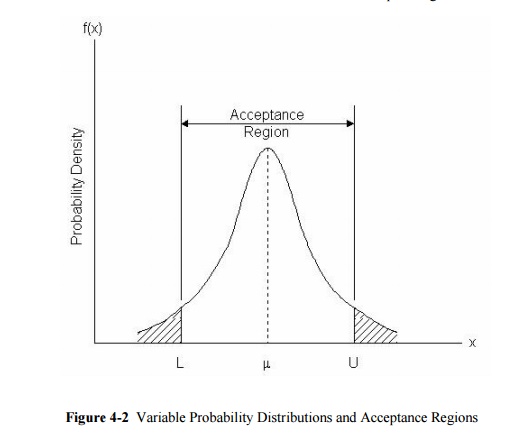
In applying sampling by variables, an acceptable
lot quality can be defined with respect to an upper limit U, a lower limit L,
or both. With these boundary conditions, an acceptable quality level can be
defined as a maximum allowable fraction of defective items, M. In Figure 13-2,
the probability distribution of item attribute x is illustrated. With an upper
limit U, the fraction of defective items is equal to the area under the
distribution function to the right of U (so that x ![]() U). This fraction of defective items would be
compared to the allowable fraction M to determine the acceptability of a lot.
With both a lower and an upper limit on acceptable quality, the fraction
defective would be the fraction of items greater than the upper limit or less
than the lower limit. Alternatively, the limits could be imposed upon the
acceptable average level of the variable.
U). This fraction of defective items would be
compared to the allowable fraction M to determine the acceptability of a lot.
With both a lower and an upper limit on acceptable quality, the fraction
defective would be the fraction of items greater than the upper limit or less
than the lower limit. Alternatively, the limits could be imposed upon the
acceptable average level of the variable.
In sampling by variables, the fraction
of defective items is estimated by using measured values from a sample of
items. As with sampling by attributes, the procedure assumes a random sample of
a give size is obtained from a lot or batch. In the application of sampling by
variables plans, the measured characteristic is virtually always assumed to be
normally distributed as illustrated in Figure 13-2. The normal distribution is
likely to be a reasonably good assumption for many measured characteristics
such as material density or degree of soil compaction. The Central Limit
Theorem provides a general support for the assumption: if the source of
variations is a large number of small and independent random effects, then the
resulting distribution of values will approximate the normal distribution. If
the distribution of measured values is not likely to be approximately normal,
then sampling by attributes should be adopted. Deviations from normal
distributions may appear as skewed or non-symmetric distributions, or as
distributions with fixed upper and lower limits.
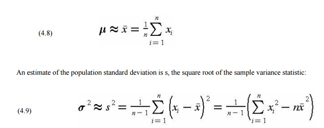
The fraction of defective items in a sample or the
chance that the population average has different values is estimated from two
statistics obtained from the sample: the sample mean and standard deviation.
Mathematically, let n be the number of items in the sample and xi, i
= 1,2,3,...,n, be the
measured values of the variable characteristic x. Then an
estimate of the overall population mean m is the sample mean:
Based on these two estimated parameters and the desired
limits, the various fractions of interest for the population can be calculated.
The probability that the average value of a population is
greater than a particular lower limit is calculated from the test statistic:
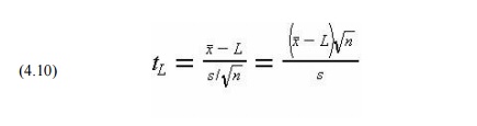
which is t-distributed with n-1 degrees of freedom. If the
population standard deviation is known in advance, then this known value is
substituted for the estimate s and the resulting test statistic would be
normally distributed. The t distribution is similar in appearance to a standard
normal distribution, although the spread or variability in the function
decreases as the degrees of freedom parameter increases. As the number of
degrees of freedom becomes very large, the t-distribution coincides with the
normal distribution.
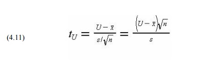
With an upper limit, the calculations are similar, and the
probability that the average value of a population is less than a particular
upper limit can be calculated from the test statistic:
With both upper and lower limits, the sum of the probabilities
of being above the upper limit or below the lower limit can be calculated.
The
calculations to estimate the fraction of items above an upper limit or below a
lower limit are very
similar to those for the population average. The only
difference is that the square root of the number of samples does not appear in
the test statistic formulas:
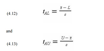
where tAL
is the test statistic for all items with a lower limit and tAU is
the test statistic for all items
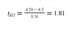
with a upper limit. For example, the test statistic for items
above an upper limit of 5.5 with ![]() = 4.0, s = 3.0, and n = 5 is tAU =
(8.5 - 4.0)/3.0 = 1.5 with n - 1 = 4 degrees of freedom.
= 4.0, s = 3.0, and n = 5 is tAU =
(8.5 - 4.0)/3.0 = 1.5 with n - 1 = 4 degrees of freedom.
Instead of using sampling plans that specify an
allowable fraction of defective items, it saves computations to simply write
specifications in terms of the allowable test statistic values themselves. This
procedure is equivalent to requiring that the sample average be at least a
pre-specified number of standard deviations away from an upper or lower limit.
For example, with ![]() = 4.0, U = 8.5, s = 3.0 and n = 41, the sample
mean is only about (8.5 - 4.0)/3.0 = 1.5 standard deviations away from the
upper limit.
= 4.0, U = 8.5, s = 3.0 and n = 41, the sample
mean is only about (8.5 - 4.0)/3.0 = 1.5 standard deviations away from the
upper limit.
To summarize, the application of sampling by
variables requires the specification of a sample size, the relevant upper or
limits, and either (1) the allowable fraction of items falling outside the
designated limits or (2) the allowable probability that the population average
falls outside the designated limit. Random samples are drawn from a pre-defined
population and tested to obtained measured values of a variable attribute. From
these measurements, the sample mean, standard deviation, and quality control
test statistic are calculated. Finally, the test statistic is compared to the
allowable trigger level and the lot is either accepted or rejected. It is also
possible to apply sequential sampling in this procedure, so that a batch may be
subjected to additional sampling and testing to further refine the test
statistic values.
With sampling by variables, it is notable that a producer of
material or work can adopt two general strategies for meeting the required
specifications. First, a producer may insure that the average quality level is
quite high, even if the variability among items is high. This strategy is
illustrated in Figure 4-3 as a "high quality average" strategy.
Second, a producer may meet a desired quality target by reducing the
variability within each batch. In Figure 4-3, this is labeled the "low
variability" strategy. In either case, a producer should maintain high
standards to avoid rejection of a batch.
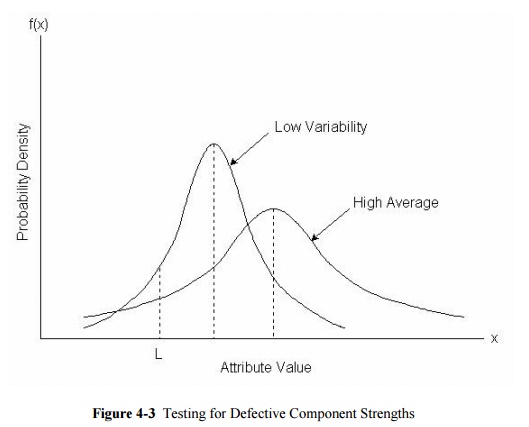
Example 4-5: Testing for defective component
strengths
Suppose
that an inspector takes eight strength measurements with the following results:
4.3, 4.8,
4.6, 4.7, 4.4, 4.6, 4.7, 4.6
In this case, the sample mean and standard deviation can be
calculated using Equations (13.8) and (13.9):
x = 1/8(4.3 + 4.8 + 4.6 + 4.7 + 4.4 + 4.6 + 4.7 +
4.6) = 4.59
s2=[1/(8-1)][(4.3 - 4.59) 2 + (4.8 -
4.59)2 + (4.6 - 4.59)2 + (4.7 - 4.59)2 + (4.4 -
4.59)2 + (4.6 - 4.59)2 + (4.7 - 4.59)2 + (4.6
- 4.59)2] = 0.16
The percentage of items below a lower quality limit of L = 4.3
is estimated from the test statistic tAL in Equation (13.12):
Related Topics