Standardizing Methods: Standard Additions

Standard Additions

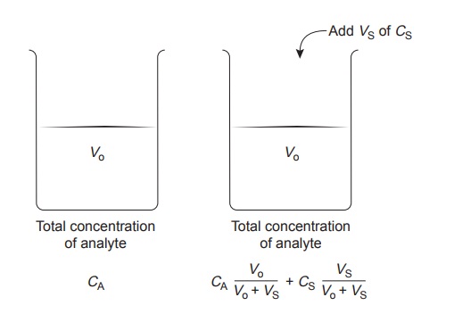
The complication of matching the matrix of the standards to that of the sample can be avoided by conducting the standardization in the sample. This is known as the method of standard additions. 

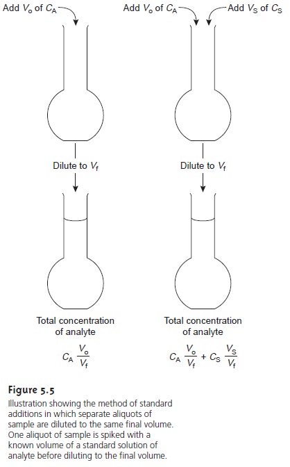
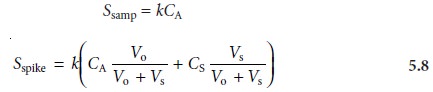
The simplest version of a standard addition is shown in Figure 5.5. A volume, V_o, of sample is diluted to a final volume, V_f, and the signal, S_samp is measured. A second identical aliquot of sample is spiked with a volume, V_s, of a standard solution for which the analyte’s concentration, C_S, is known. The spiked sample is diluted to the same final volume and its signal, S_spike, is recorded. The following two equations relate S_samp and S_spike to the concentration of analyte, C_A, in the original sample

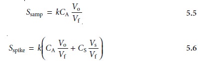
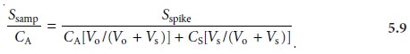
where the ratios V_o/V_f and V_s/V_f account for the dilution. As long as V_s is small rela- tive to V_o, the effect of adding the standard to the sample’s matrix is insignificant, and the matrices of the sample and the spiked sample may be considered identical. Under these conditions the value of k is the same in equations 5.5 and 5.6. Solving both equations for k and equating gives

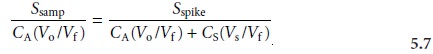
Equation 5.7 can be solved for the concentration of analyte in the original sample.

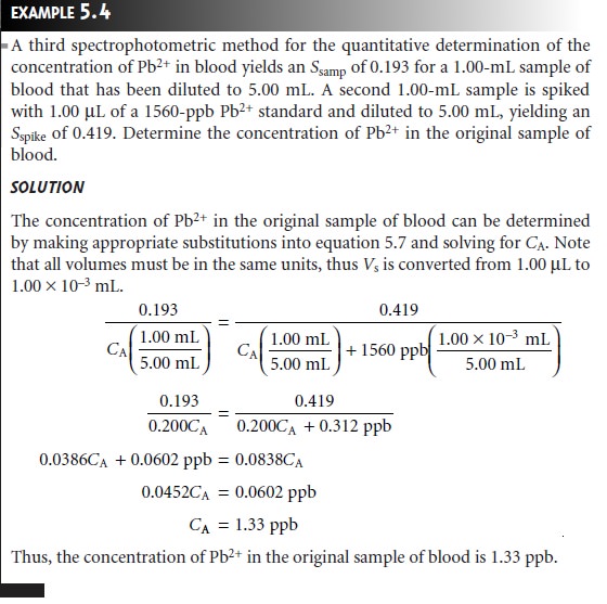
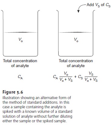
It also is possible to make a standard addition directly to the sample after mea- suring S_samp (Figure 5.6). In this case, the final volume after the standard addition is V_o + V_s and equations 5.5–5.7 become

The single-point standard additions outlined in Examples 5.4 and 5.5 are easily adapted to a multiple-point standard addition by preparing a series of spiked sam- ples containing increasing amounts of the standard. A calibration curve is prepared by plotting S_spike versus an appropriate measure of the amount of added standard. Figure 5.7 shows two examples of a standard addition calibration curve based on equation 5.6. In Figure 5.7(a) S_spike is plotted versus the volume of the standard so- lution spikes, V_s. When k is constant, the calibration curve is linear, and it is easy to show that the x-intercept’s absolute value is C_AV_o/C_S.

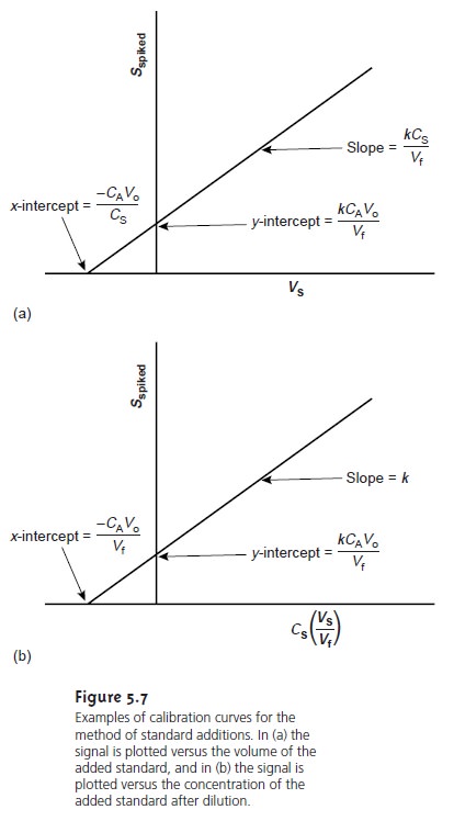
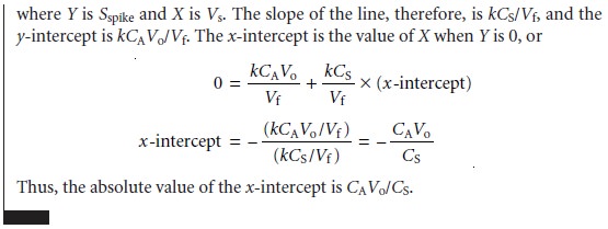
 Since both V_o and C_S are known, the x-intercept can be used to calculate the analyte’s concentration.

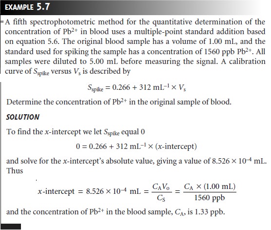
Figure 5.7(b) shows the relevant relationships when S_spike is plotted versus the con- centrations of the spiked standards after dilution. Standard addition calibration curves based on equation 5.8 are also possible.

Since a standard additions calibration curve is constructed in the sample, it cannot be extended to the analysis of another sample. Each sample, therefore, re- quires its own standard additions calibration curve. This is a serious drawback to the routine application of the method of standard additions, particularly in labora- tories that must handle many samples or that require a quick turnaround time. For example, suppose you need to analyze ten samples using a three-point calibration curve. For a normal calibration curve using external standards, only 13 solutions need to be analyzed (3 standards and 10 samples). Using the method of standard additions, however, requires the analysis of 30 solutions, since each of the 10 sam- ples must be analyzed three times (once before spiking and two times after adding successive spikes).

The method of standard additions can be used to check the validity of an exter- nal standardization when matrix matching is not feasible. To do this, a normal cali- bration curve of S_stand versus C_S is constructed, and the value of k is determined from its slope. A standard additions calibration curve is then constructed using equation 5.6, plotting the data as shown in Figure 5.7(b). The slope of this standard additions calibration curve gives an independent determination of k. If the two val- ues of k are identical, then any difference between the sample’s matrix and that of the external standards can be ignored. When the values of k are different, a propor- tional determinate error is introduced if the normal calibration curve is used.