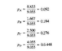
Chapter: Automation, Production Systems, and Computer Integrated Manufacturing : Flexible Manufacturing Systems
QuantitativeAnalysisof Flexible Manufacturing Systems
QUANTITATIVE ANALYSIS OF FLEXIBLE MANUFACTURING SYSTEMS
QuantitativeAnalysisof Flexible Manufacturing Systems:
a. Bottleneck Model
b. Extended Bottleneck Model
c. Sizing the FMS
d. What the Equations Tell Us
Most of the design and operational problems identified in Section 16.4 can be addressed using quantitative analysis techniques. FMSs have constituted an active area of interest in operations research, and many of the important contributions are included in our list of references. FMS analysis techniques can be classified as follows: (l) deterministic models, (2) queuing models, (3) discrete event simulation, and (4) other approaches, including heuristics.
To obtain starting estimates of system performance, deterministic models can be used. Later :n this section, we present a deterministic modeling approach that is useful in the beginning stages of FMS design to provide rough estimates of system parameters such as production rate, capacity, and utilization. Deterministic models do not permit evaluation of operating characteristics such as the buildup of queues and other dynamics that can impair performance of the production system. Consequently, deterministic models tend to overestimate FMS performance. On the other hand, if actual system performance is much lower than the estimates provided by these models, it may be a sign of either poor system design or poor management of the FMS operation.
Queueing models can be used to describe some of the dynamics not accounted for in deterministic approaches. These models are based on the mathematical theory of queues ["hey permit the inclusion of queues, but only in a general way and for relatively simple sys· tern configurations. The performance measures that are calculated are usually average values for steady-state operation of the system. Examples of queueing models to study FMS, include, Probably the most well known of the FMS queueing models is CAN-Q.
In the later stages of design, discrete event simulation probably offers the most accurate method for modeling the specific aspects of a given FMS [28], [45]. The computer model can be constructed to closely resemble the details of a complex FMS operation Characteristics such as layout configuration, number of pallets in the system. and production scheduling rules can be incorporated into the FMS simulation model. Indeed, the simulation can be helpful in determining optimum values for these parameters
Other techniques that have been applied to analyze £OMS design and operational problems include mathematical programming [34] and various heuristic approaches [I], [17]. Several literature reviews on operations research techniques directed at FMS problems are included among our references, specifically [2], [6], [20], and [37].
Bottleneck Model
Important aspects of FMS performance can be mathematically described by a deterministic model called the bottleneck model, developed by Solberg [33] Notwithstanding the limitations of a deterministic approach, the value of the bottleneck model is that it is simple and intuitive. It can be used to provide starting estimates of FMS design parameters such as production rate and number of workstations. The tenn bottleneck refers 10 the faci that the output of the production system has an upper limit, given that the product mix flowing through the system is fixed. The model can be applied to any production system that possesses this bottleneck feature, for example, a manually operated machine cell or a production job shop. It is not limited to FMSs.
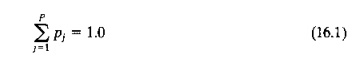
Terminology and Symbols. Let us define the features, terms, and symbols for the bottleneck model as they might be applied to an FMS:
Part mix. The mix of the various part or product styles produced by the system is defined b) "PI' .••••here PJ ' the fraction of the total system output that is of style j.The sub-script j = 1,2, .. ,P, where P = the total number of different part styles made in the FMS during the time period of interest. The values of Pi must sum to unity; that is.
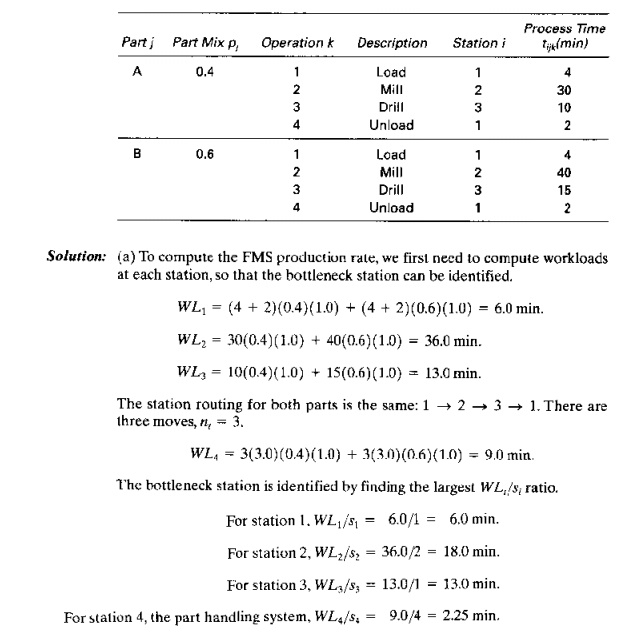
Workstations and servers. The flexible production system has a number of distinctly different workstations n. In the terminology of the bottleneck model, each workstation may have more than one server, which simply means that it is possible to have two or more machines capable of performing the same operations. Using the terms "stations" and "servers" in the bottleneck model is a precise way of distinguishing
between machines that accomplish identical operations from those that accomplish different operations. Let Si = the number of servers at workstation i, where i = 1,2. , n, We include the load/unload station as one of the stations in the FMS
Process routing. For each part or product, the process routing defines the sequence of operations. the workstations at which they are performed, and the associated processing times. The sequence includes the loading operation at the beginning of proon the FMS and the unloading operation at the end of processing. Let tijk = processing time, which is the total time that a production unit occupies a given workstation server, not counting any waiting time at the station. In the notation for tijk, the Subscript I refers to the station, j refers to the part or product, and k refers to the sequence of operations in the process routing. For example, the fourth opera. non in the process plan for part A is performed on machine 2 and lakes 8.5 min; thus, t = 8.5 min. Note that process plan j is unique to part j. The bottleneck model does not conveniently allow for alternative process plans for the same part.
Work handling system. The material handling system used to transport parts or products within the FMS can be considered to be a special case of a workstation. Let us designate it as station n + 1, and the number of carriers in the system (e.g., conveyor carts, AGVs, monorail vehicles, etc.) is analogous to the number of servers in a regular workstation. Let sn~1 "" the number of carriers in the FMS handling system
Transport time. Let tijk = the mean transport time required to move a part from one workstation to the next station in the process routing. This value could be computed for each individual transport based en transport velocity and distances between stations in the FMS, but it is more convenient to simply use an average transport time for all moves in the FMS.
Operation frequency. The operation frequency is defined as the expected number of times a given operation in the process routing is performed for each work unit. For example, an inspection might be performed on a sampling basis. once every four units; hence, the frequency for this operation would he 0.25. In other cases, the part may have an operation frequency greater than 1.0;for example. for a calibration procedure that
have to be performed more than once on average to be completely effective. ' The operation frequency for operation k in process plan jat station i
FMS Operational Parameters. Using the above terms, we can next define certain average operational parameters of the production system. The average workload for a given station is defined as the mean total time spent at the station per part. It is calculated as follows
where WL = average workload for station i (min),tijk = processing time for operation k in process pian i at station i (min),fijk =operation frequency for operation k in part j at station t and Pj = part mix fraction for part j.
The work handling system (station n + 1) is a special case as noted in our terminology above. The workload of the handling system is the mean transport time multiplied by the average number of transports required to complete the processing of a workpart. The average number of transports is equal to the mean number of operations in the process routing minus one. That is,
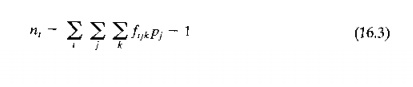
where nt mean number of transports. and the other terms are defined above. Let us illustrate this with a simple example
EXAMPLE 16.6 Determining /1,
Consider a manufacturing system with two stations: (1) a load/unload station and (2) a machining station. There is just one part processed through the production system, part A, 50 the part mix fraction PA == LO. The frequency of all operations is fAK = 1.0. The parts arc loaded at station 1, routed to station 2 for machining, and then sent hack to stauon 1 for unloading (three operations in the routing).11singEq.(16.3).

Looking at it another way. the process routing is (1) -- > t (2) -- > t (1). Counting the number of arrows gives us the number of transports: n, = 2.
We are now in a position to compute the workload of the handling system:
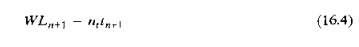
where", WLn+1 = workload of the handling system (min), nt, = mean number of transports by Eq. (16.3) and tn-1 = mean transport time per move (min).
System Performance Measures. Important measures for assessing the performance of an FMS include production rate of all parts. production rate of each part style, utilization of the different workstations, and number of busy servers at each workstation.
These measures can be calculated under the assumption that the FMS is producing at its maximum possible rate. This rate is constrained by the bottleneck station in the system, which is the station with the highest workload per server. The workload per server is simply the ratio WL,/s, for each station. Thus the bottleneck is identified by finding the maximum value of the ratio among all stations. The comparison must include the handling system, smce it might be the bottleneck in the system.
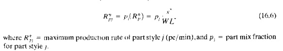
Let W L* s*, and t'" equal the workload, number of servers, and processing time, respectively, for the bottleneck. station. The FMSmaximum production rate of all parts can he determined as the ratio of s* to W L* . Let us refer to it as the maximum production rate because it is limited by the capacity of the bottleneck station.
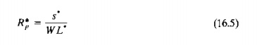
where R; = maximum production rate of all part styles produced by the system, which is determined by the capacity of the bottleneck station (pc/rnin}, s* = number of servers at the bottleneck station, and W L* = workload at the bottleneck station (min/pc). It is not difficult to grasp the validity of this formula as long as all parts are processed through the bottleneck station. A little more thought is required to appreciate that Eq. (16.5) is also valid, even when not all of the parts pass through the bottleneck station, as long as the product mix (PI values) remains constant. In other words, if we disallow those parts not passing through the bottleneck from increasing their production rates to reach their respective bottleneck limits. these parts will be limited by the part mix ratios
The value of R* include, parts of all styles produced in the system. Individual pari production rates can be obtained by multiplying R~ by the respective part mix ratios. That is,
mean utilization of each workstation is the proportion of time that the servers at the station are working and not idle. This can be computed as follows:
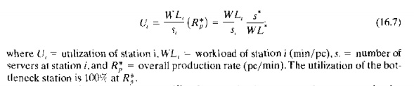
To obtain the average station utilization, one simply computes the average value for all stations. including the transport system. This can he calculated as follow,
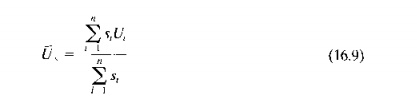
where U is an unweighted average of the workstation utilizations.
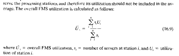
A more useful measure of overall FMS utilization can be obtained using a weighted average. where the weighting is based on the number of servers at each station for the n regular stations in the system. and the transport system IS omitted from the average. Theargument for omitting the transport system is that the utilization of the processing stations is the important measure of FMS utilization. The purpose of the transport system is to
Finally, the number of busy servers at each station is of interest. All of the servers at the bottleneck station are busy at the maximum production rate, but the servers at the other stations are idle some of the time, The values can be calculated as follows
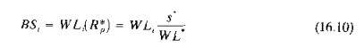
where BSi= number of busy servers on average at station i, and WLt = workload at station i
Let us present two example problems to illustrate the bottleneck model, the first a simple example whose answers can be verified intuitively, and the second a more complicated problem.
EXAMPLE 16.7 Bottleneck model on a simple problem
A flexible machining system consists of two machining workstations and a load/unload station. Station 1 is the load/unload station. Station 2 performs milling operations and consists of two servers (two identical CNC milling machines). Station 3 has one server that performs drilling (one CNC drill press). The stations are connected by a part handling system that has four work carriers. The mean transport time is 3.0 min. The FMS produces two parts,A and B. The part mix fractions and process routings for the two parts are presented in the table below. The operation frequency fijk = 1.0 for all operations. Determine: (a) maximum production rate of the FMS, (b) corresponding production rates of each product, (c) utilization of each station, and (d) number of busy servers at each station.
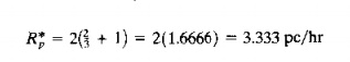
The maximum ratio occurs at station 2, so it is the bottleneck station that determines the maximum production rate of all parts made by the system.
Rp* = 2/36.0 = 0.05555 pc/min = 3.333 pc/hr
(b) To determine production rate of each product, multiply R; by its respective part mix fraction.
R*pA = 3.333(0.4) = 1.333 pc/hr
R*pB = 3.333(0.6) = 2.00 pc/hrr
(c) The utilization of each station can be computed using Eq. (16.7):
U1 | = (6,0/1)(0.05555) | =0.333 | (33.3%) | |
U2 | = (36.0/2)(0.05555) | = | 1.0 | (100%) |
U3 | =(13.0/1)(0.05555) | = | 0.722 | (72.2%) |
U4 | = (9,Oj4)(0.05555) | = 0.125 | (12.5%) | |
(d) Mean number of busy servers at each station is determined using Eq. (16.10):
BSj = 6.0(0.05555) = 0.333
BS2 = 36,0(0.05555) = 2.0
B53 = 13.0(0.05555) = 0.722
BS4 = 9.0(0.05555) = 0.50
We designed the preceding example so that most of the results could be verified without using the bottleneck model. For example, it is fairly obvious that station 2 is the limiting station, even with two servers. The processing times at this station are more than twice those at station 3. Given that station 2 is the bottleneck, let us try 10 verify the maximum production rate of the FMS. To do this, the reader should note that the processing times at station 2 are t2A2 = 30 min and 12B2 = 40 min. Note also that the part mix fractions
0.4 and PR = 0.6. This means that for every unit of R produced, there are 1 units of part A. The corresponding time to process 1 unit of Band j unit of A at station 1 is
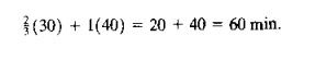
Sixty minutes is exactly the amount ~f processing time each machine has available in an hour. (This is no coincidence; we designed the problem so this would happen.) With two servers (two CNC mills), the FMS can produce parts at the following maximum rate:
This is the same result obtained by the bottleneck model. Given that the bottleneck station is working at 100% utilization, it is easy to determine the utilizations of the other stations. At station 1, the time needed 10 load and unload the output of the two servers at station 2 is
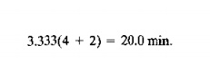
As a fraction of 60 min. in an hour, this gives a utilization of Vj = OJ33. AI station 3, the processing time required to process the output of the two servers at station 2 is
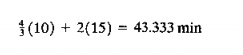
As a fraction of the 60 min., we have U3 = 43.333/60 = 0.722. Using the same approach on the part handling system, we have
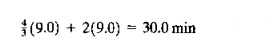
As a fraction of 60 min, this is 0.50. However, since there are four servers (four work carriers), this fraction is divided by 4 to obtainU4 = 0.125. These are the same utilization values as in our example using the bottleneck model.
EXAMPLE 16.8 Bottleneck Model on a more complicated Problem
An FMS consists of four stations. Station 1 is a load/unload station with one server. Station 2 performs milling operations with three servers (three identical CNC milling machines). Station 3 performs drilling operations with two servers (two identical CNC drill presses). Station 4 is an inspection station with one server that performs inspections on a sampling of the parts. The stations are connected by a part handling system that has two work carriers and whose mean transport time = 35 min. The FMS produces four parts. A, B, C, and D. The part mix fractions and process routings for the four parts are presented in the table below. Note that the operation frequency at the inspection station (f4jk) is less than 1.0 to account for the fact that only a fraction of the parts are inspected. Determine: (a) maximum production rate of the FMS, (b) corresponding production rate of each part, (e) utilization of each station in the system, and (d) the overall FMS utilization.
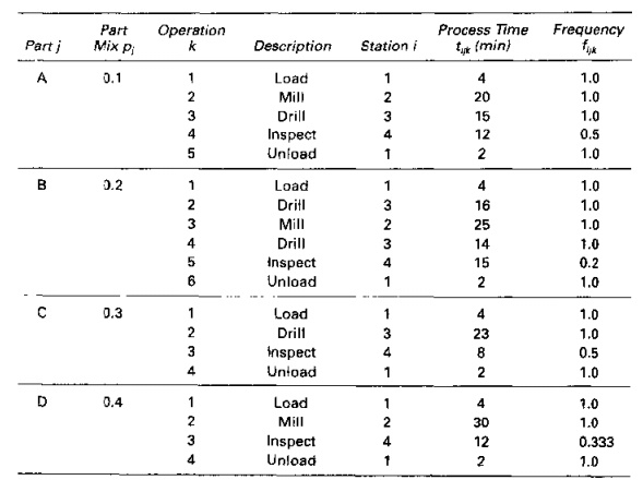
Solution: (a) We first calculate the workloads at the workstations to identify the bottleneck station
WLI = (4 + 2)(1.0)(0.1 + Q.2 + 0.3 + 0.4) == 6.0 min.
WL2 = 20(1.0)(0.1) + 25(1.0){0.2) + 30(1.0)(0.4) = 19.0 min.
WL3 = 15(1.0)(0.1) + 16(1.0)(0.2) + 14(1.0)(0.2) + 23(1.0)(0.3) = 14.4 min
WL4 = 12{0.5)(0.1) + 15(0.2)(0.2) + 8(0.5)(0.3) + 12(0.333)(0.4) = 4.0 min.
nJ = (3.5)(0.1) + (4.2)(0.2) + (2.5)(0.3) + (2.333)(0.4) = 2.873
WL, = 2.873(3.5) = 10.06 min.
The bottleneck station is identified by the largest W Ljs ratio:
For station I, WLjjSI = 6.0j1 = 6.0
For station 2, WLzjS2 == 19.0/3 = 6.333
For station 3, WLJ!Sl = 14.4/2 = 7.2
For station 4, WL4jS4 = 4.0j1 = 4.0
For the part handling system, WLs/ss = 10.06;2 == 5.03
The maximum ratio occurs at station 3, so it is the bottleneck station that determines the maximum rate of production of the system
R*p = 2/14.4 == 0.1389 pc/min = 8.333 pc/hr
To determine the production rate of each product, multiply R; by its respective part mix fraction
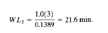
R*pA = 8.333(0.1) = O.8333pc/hr
R*pB = 8.333(0.2) = 1.667 pc/hr
R*pC '" R.333(0.3) = 2.500pcjhr
R*pD = 8.333(0.4) = 3.333 pc/hr
(e) Utilization of each station can be computed using Eq. (16.7)'
U1 = (6.0/1)(0.1389) = 0.833 (83.3%)
U2 = (19.0;3)(0.1389) = 0.879 (87.9%)
U3 (14.4/2)(0.1389) ~ 1.000 (100%)
U4 = (4.0/1)(0.1389) = 0.555 (55.5%)
U5 = (1O.06j2)(O,1389) = 0.699 (69.9%)
Overall FMS utilization can be determined using a weighted average of the above values, where the weighting is based on the number of servers per station and the part handling system is excluded from the average, as ill Eq. (16.9)'
U, = [ 1(0.833) + 3(0.879)/ 2(1.0) + 1(0.555j ] /7= 0.861 (86.1%)
In the preceding example, it should be noted that the production rate of part D is constrained by the part mix fractions rather than the bottleneck station (station 3). Part D is not even processed on the bottleneck station. Instead, it is processed through station 2, which has unutilized capacity. It should therefore be possible to increase the output rate of part D by increasing its part mix fraction and at the same time increasing the utilization of station 2 to 100%. The following example illustrates the method for doing this.
EXAMPLE 16.9 Increasing Unutilized Station Capacity
From Example 16.8, V2 = 87.9%.Determine the production rate of part D that will increase the utilization of station 2 to 100%.
Solution: Utilization of a workstation is calculated using Eq.16.7. For station 2:
Setting the utilization of station 2 to 1.0 (100%), we can solve for the corresponding W Lz value.
This compares with the previous workload value of 19.0 min computed in Example 16.8. A portion of the workload for both values is accounted for by parts A and R This portion is

WL2(A + B) = 20(0.1)(1.0) + 25(0.2)(1.0) = 7.0 min.
The remaining portions of the workloads are due to part D.
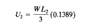
For the workload at 1001(, utilization, WL2(D) = 21.6 7.0 = 14.6 min.
For the workload at 87.9% utilization, WL2D) = 19.0 7.0 = 12.0 min
We can now use the ratio of these values to calculate the new (increased) production rate for part D:
RpD = ~~:~ (3.333) = 1.2167(3.333) = 4.055 pc/hr
Production rates of the other three products remain the same as before. Accordingly, the production rate of all parts increases to the following:
R; = 833 + 1.667 + 2.500 + 4.055 = 9.055 pc/hr.
Although the production rates of the other three products are unchanged, the increase in production rate for parts D alters the relative part mix fractions. The new values are:
Extended Bottleneck Model
The bottleneck model assumes that the bottleneck station is utilized 100% and that there are no delays in the system due to queues. This implies on the one hand that there are a sufficient number of parts in the system to avoid starving of workstations and on the other hand that there will be no delays due to queueing. Solberg [33J argued that the assumption of 100% utilization makes the bottleneck model overly optimistic and that a queueing model that accounts for process time variations and delays would more realistically and completely describe the performance of an FMS.
An alternative approach, developed by Mejabi [25], addresses some of the weaknesses of the bottleneck model without resorting to queueing computations (which can be difficult, sometimes even worse). He called his approach the extended bottleneck model This extended model assumes a closed queueing network in which there are always a certain number of workparts in the FMS. Let N = this number of parts in the system. When one part is completed and exits the FMS, a new raw workpart immediately enters the system, so tbar N remains constant. The new part mayor may not have the same process routing as the one just departed. The process routing of the entering part is determined according to probabilities Pi
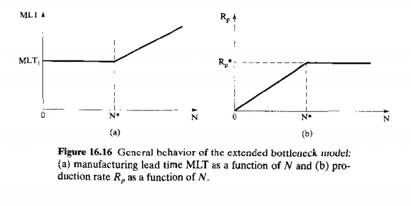
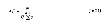
N plays a critical role in the operation of the production system. If N is small (say. much smaller than the number of workstations), then some of the stations will be idle due to starving, sometimes even the bottleneck station. In this case, the production rate of theFMS will be less than R~ calculated in Eq. (16.5).lf N is large (say, much larger than the number of workstations), then the system will be fully loaded, with queues of parts waiting in front of the stations. In this case, R*p will provide a good estimate of the production capacity of the system. However, WIP will be high, and manufacturing lead time (MLT) will belong.
In effect, WIP corresponds to N, and MLT is the sum of processing times at the workstations, transport times between stations, and any waiting time experienced by the parts in the system. We can express MLT as follows:
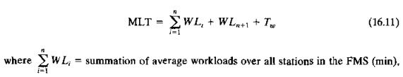
= summation of average workloads over all stations in the FMS (min).
WLn+1 = workload of the part handling system (min), and Tw = mean waiting time experienced by a part due to queues at the stations (min).
WIP (that is, N) and MLT are correlated. If N is small, then MLT will take on its smallest possible value because waiting time will be short (zero). If N is large, then MLT will be long and there will be waiting time in the system. Thus we have two alternative cases that must be distinguished, and adjustments must be made in the bottleneck model to account for them. To do this, Mejabi found the wellknown Little's formula" from queueing theory to be useful. Little's formula establishes the relationship between the mean expected time a unit spends in the system, the mean processing rate of items in the system, and the mean number of units in the system. It can be mathematically proved for a single station queueing system, and its general validity is accepted for multi-station queueing systems. Using our own symbols, Little's formula can be expressed as follows:
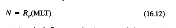
where N = number of parts in the system (pc), Rp = production rate of the system (pc/min), and MLT = manufacturing lead time (time spent in the system by a part) (min). Now, lei us examine the two cases:
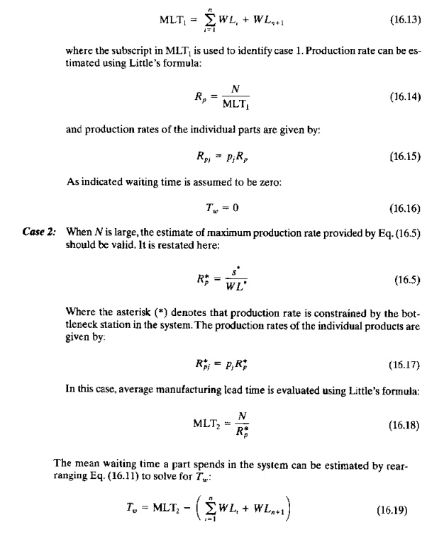
The decision whether to use case 1 or case 2 depends on the value of N. The dividing line between cases 1 and 2 is determined by whether N is greater than or less than a critical value given by the following:
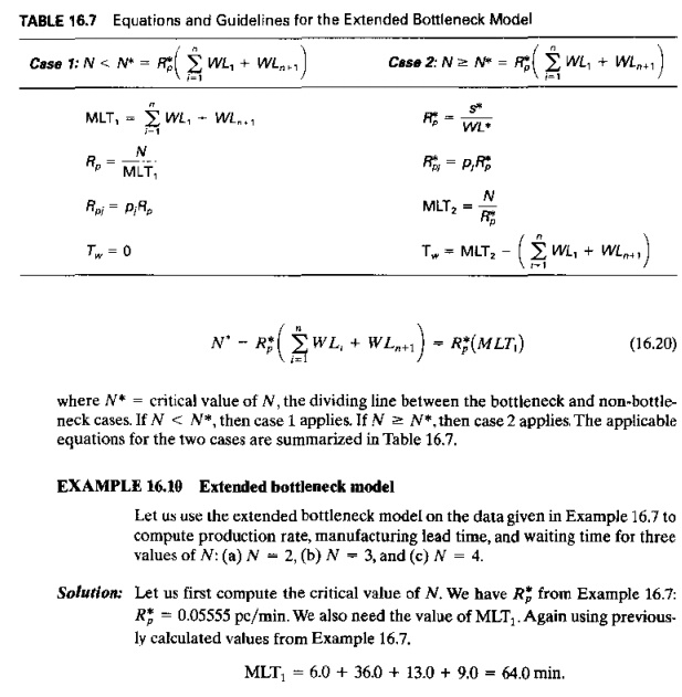
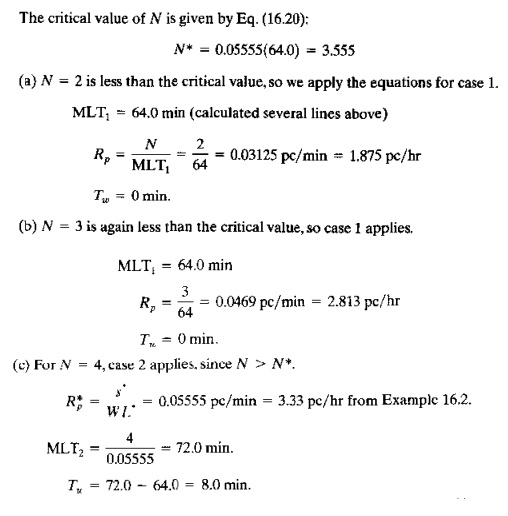
The results of this example typify the behavior of the extended bottleneck model, shown in Figure 16.16. Below N* (case 1), MLT has a constant value, and Rp decreases proportionally as N decreases. Manufacturing lead time cannot be less than the sum of the processing and transport times, and production rate is adversely affected by low values of N because stations become starved for work. Above N* (case 2), Rp has a constant value equal to R; and MLT increases. No matter how large N is made, the production rate cannot be greater than the output capacity of the bottleneck station. Manufacturing lead time increases because backlogs build up at the stations.
The preceding observations might tempt us to conclude that the optimum N value occurs at N*, since MLT is at its minimum possible value, and Rp is at its maximum possible value. However, caution must be exercised in the use of the extended bottleneck model (and the same caution applies even more so to the conventional bottleneck model, which disregards the effect of N)_lt is intended to be a rough-cut method to estimate FMS performance in the early phases of FMS design. More reliable estimates of performance can be obtained using computer simulations of detailed models of the FMS models that include considerations of layout, material handling and storage system, and other system design factors.
Mejabi compared the estimates computed using the extended bottleneck model with estimates obtained from the CANQ model [32], [33] for several thousand cases. He developed an adequacy factor to assess the differences between the extended bottleneck model and C ANQ. The adequacy factor is computed'
carriers in the transport system. The anticipated discrepancies corresponding to the value of AF are tabulated in Table 16.8. It is likely that an FMS would be scheduled so that the number of parts in the system is somewhat greater than the number of servers. This would result in adequacy factor values greater than 1.5, permitting the extended bottleneck model to provide estimates of production rate and manufacturing lead time that agree fairly closely with those computed by CANQ
Sizing the FMS
The bottleneck model can be used to calculate the number of servers required at each workstation to achieve a specified production rate. Such calculations would be useful during the initial stages of FMS design in determining the "size" (number of workstations and servers) of the system. The starting information needed to make the computation consists of part mix, process routings, and processing times so that workloads can be calculated for each of the stations to be included in the FMS. Given the workloads, the number of servers at each station i is determined as follows:
EXAMPLE 16.11 Sizing the FMS
Suppose the part mix, process routings, and processing times for the family of parts to be machined on a proposed FMS are those given in Example 16.8. Determine how many servers at each station i will be required to achieve an annual production rate of 60,000 parts/yr. The FMS will operate 24 hr/day, 5 day/wk. 50 wk/yr. Anticipated availability of the system is 95%.
Solution: The number of hours of FMS operation per year will be 24 X 5 X 50 = 6000 hr/yr. Taking into account the anticipated system availability, the average hourly production rate is given by:
Because the number of servers at each workstation must be an integer. station utilization may be less than 100% for most if not all of the stations. In Example 16.11, all of the stations have utilizations less than 100%. The bottleneck station in the system is identified as the station with the highest utilization, and if that utilization is less than 100%, the maximum production rate ofthe system can be increased until U* = 1.0, The following example illustrates the reasoning.
EXAMPLE 16.12 Increasing Utilization and Production Rate at the Bottleneck Station
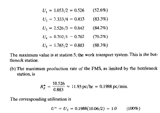
For the specified production rate in Example 16.11, determine: (a) the utilizations for each station and (b) the maximum possible production rate at each station if the utilization of the bottleneck station were increased 10 100%.
Solution: (a) The utilization at each workstation is determined as the calculated value of s, divided by the resulting minimum integer value >=si
What the Equations Tell Us
Notwithstanding its limitations, the bottleneck model and extended bottleneck model provide some practical guidelines for the design and operation of FMSs. These guidelines can be expressed as follows:
For a given product or part mix, the total production rate of the FMS is ultimately limited by the productive capacity of the bottleneck station, which is the station with the maximum workload per server.
If the product or part mix ratios can be relaxed, it may be possible !O increase total FMS production rate by increasing the utilization of nonbottleneck workstations.
The number of parts in the FMS at any time should be greater than the number of servers (processing machines) in the system. A ratio of around 2.() parts/server is probably optimum, assuming that the parts are distributed throughout the FMS to ensure that a part is waiting at every station. This is especially critical at the bottleneck station.
If WIP (number of parts in the system) is kept at too Iowa value, production tate of the system is impaired.
If WIP is allowed to be too high, then manufacturing lead time will be long with no improvement in production rate.
As a first approximation. the bottleneck model can be used to estimate the number of servers at each station (number of machines of each type) to achieve a specified overall production rate of the system.
Related Topics