Additional Simplex Algorithms: Dual Simplex Method and Generalized Simplex Algorithm

ADDITIONAL SIMPLEX ALGORITHMS

In the simplex algorithm presented in Chapter 3 the problem starts at a (basic) feasible solution. Successive iterations continue to be feasible until the optimal is reached at the last iteration. The algorithm is sometimes referred to as the primal simplex method.

This section presents two additional algorithms: The dual simplex and the generalized simplex. In the dual simplex, the LP starts at a better than optimal infeasible (basic) solution. Successive iterations remain infeasible and (better than) optimal until feasibility is restored at the last iteration. The generalized simplex combines both the primal and dual simplex methods in one algorithm. It deals with problems that start both nonoptimal and infeasible. In this algorithm, successive iterations are associated with basic feasible or infeasible (basic) solutions. At the final iteration, the solution be-comes optimal and feasible (assuming that one exists).

All three algorithms, the primal, the dual, and the generalized, are used in the course of post-optimal analysis calculations, as will be shown in Section 4.5.

1. Dual Simplex Algorithm

The crux of the dual simplex method is to start with a better than optimal and infeasible basic solution. The optimality and feasibility conditions are designed to preserve the op-timality of the basic solutions while moving the solution iterations toward feasibility.

Dual feasibility condition. The leaving variable, x _n is the basic variable having the most negative value (ties are broken arbitrarily). If all the basic variables are nonnegative, the algorithm ends.

Dual optimality condition. Given that x_r is the leaving variable, let Bar(c_j) be the reduced cost of nonbasic variable x_j and a_rj the constraint coefficient in the x_r-row and x_j- column of the tableau. The entering variable is the nonbasic variable with a_rj < 0 that corresponds to

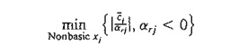
(Ties are broken arbitrarily.) If a_rj ≥ 0 for all nonbasic x_j, the problem has no feasible solution.

To start the LP optimal and infeasible, two requirements must be met:

1.     The objective function must satisfy the optimality condition of the regular simplex method (Chapter 3).

2.     All the constraints must be of the type (≤).

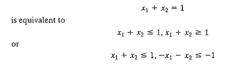
The second condition requires converting any (≥) to (≤) simply by multiplying both sides of the inequality (≥) by -1. If the LP includes (=) constraints, the equation can be replaced by two inequalities. For example,

After converting all the constraints to (≤), the starting solution is infeasible if at least one of the right-hand sides of the inequalities is strictly negative.

Example 4.4-1

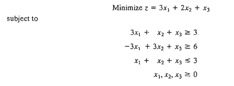
In the present example, the first two inequalities are multiplied by -1 to convert them to (≤) constraints. The starting tableau is thus given as:

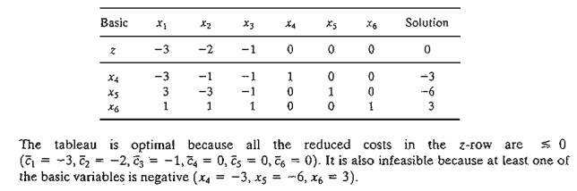
According to the dual feasibility condition, x₅ (= -6) is the leaving variable. The next table shows how the dual optimality condition is used to determine the entering variable.

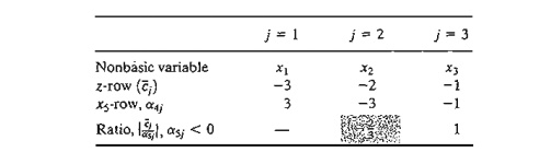
The ratios show that x₂ is the entering variable. Notice that a nonbasic variable x_j is a candidate for entering the basic solution only if its a_rj is strictly negative. This is the reason x₁ is excluded in the table above.

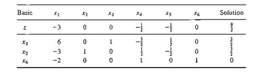
The next tableau is obtained by using the familiar row operations, which give

The preceding tableau shows that x₄ leaves and x₃ enters, thus yielding the following tableau, which is both optimal and feasible:

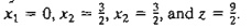
Notice how the dual simplex works. In all the iterations, optimality is maintained (all reduced costs are ≤0).At the same time, each new iteration moves the solution toward feasibility. At iteration 3, feasibility is restored for the first time and the process ends with the optimal feasible solution as

TORA Moment.

TQRA provides a tutorial          module for the  dual simplex             method.   From the SOLVE/MODIY Menu slect - > Algebraic -> Iterations - > Dual Simplex Remember that you need to convert (=) constraints to inequalities. You do not need  to convert (2:) constraints because TORA will do the conversion internally. If the LP does not satisfy the initial requirements of the dual simplex, a message will appear on the screen.

As in the regular simplex method, the tutorial module allows you to select the entering and the leaving variables beforehand. An appropriate feedback then tells you if your selection is correct.

PROBLEM SET 4.4A

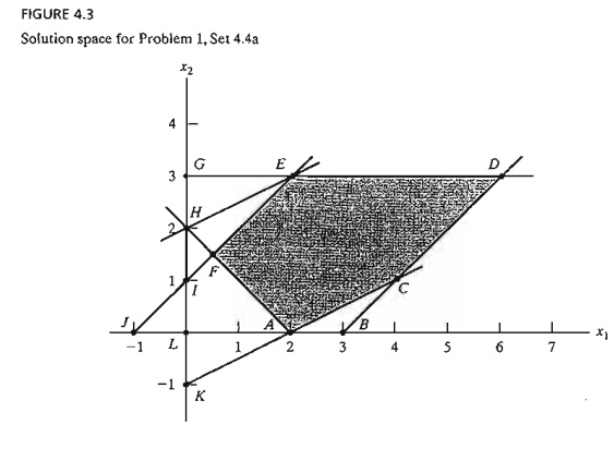
1. Consider the solution space in Figure 4.3, where it is desired to find the optimum extreme point that uses the dual simplex method to minimize z = 2x₁ + x_2. The optimal solution occurs at point F = (0.5,1.5) on the graph.

(a)        Can the dual simplex start at point A?

*(b) If the starting basic (infeasible but better than optimum) solution is given by point G, would it be possible for the iterations of the dual simplex method to follow the path G -> E -> F? Explain.

(c) If the starting basic (infeasible) solution starts at point L, identify a possible path of the dual simplex method that leads to the optimum feasible point at point F.

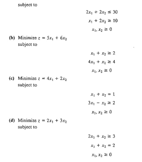
2. Generate the dual simplex iterations for the following problems (usingTORA for conve-nience), and trace the path of the algorithm on the graphical solution space.

Minimize z =  2x₁  + 3x₂

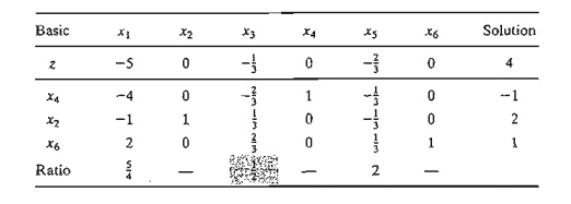
3.       Dual Simplex with Artificial Constraints. Consider the following problem:

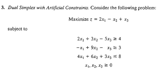
The starting basic solution consisting of surplus variables x₄ and x₅ and slack variable x₆ is infeasible because x₄ = -4 and x₅ = -3. However, the dual simplex is not applicable directly, because x₁ and x₃ do not satisfy the maximization optimality condition. Show that by adding the artificial constraint x₁ +x₃  ≤ M (where M is sufficiently large not to eliminate any feasible points in the original solution space), and then using the new constraint as a pivot row, the selection of x_l as the entering variable (because it has the most negative objective coefficient) will render an all-optimal objective row. Next, carry out the regular dual simplex method on the modified problem.

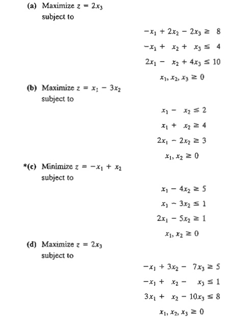
4. Using the artificial constraint procedure introduced in Problem 3, solve the following problems by the dual simplex method. In each case, indicate whether the resulting solution is feasible, infeasible, or unbounded.

5. Solve the following LP in three different ways (useTORA for convenience). Which method appears to be the most efficient computationally?

2. Generalized Simplex Algorithm

The (primal) simplex algorithm in Chapter 3 starts feasible but nonoptimal. The dual simplex in Section 4.4.1 starts (better than) optimal but infeasible. What if an LP model starts both nonoptimal and infeasible? We have seen that the primal simplex accounts for the infeasibility of the starting solution by using artificial variables. Similarly, the dual simplex accounts for the nonoptimality by using an artificial constraint (see Problem 3, Set 4.4a).Although these procedures are designed to enhance automatic computations, such details may cause one to lose sight of what the simplex algorithm truly entails-namely, the optimum solution of an LP is associated with a comer point (or basic) solution. Based on this observation, you should be able to "tailor" your own sim-plex algorithm for LP models that start both nonoptimal and infeasible. The following example illustrates what we call the generalized simplex algorithm.

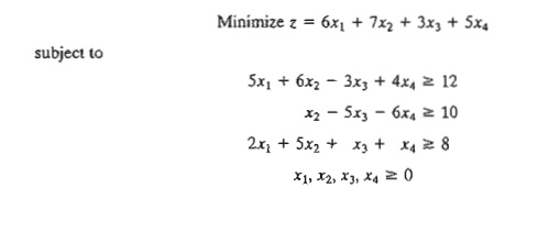
Example 4.4-2

Consider  the LP model of Problem 4(a), Set 4.4a. The model can be put in the following tableau form in which the starting basic solution (x₃, x₄, x₅) is both nonoptimal (because x₃ has a negative reduced cost) and infeasible (because x₄  =  -8). (The first equation has been multiplied by -1 to reveal the infeasibility directly in the Solution column.)

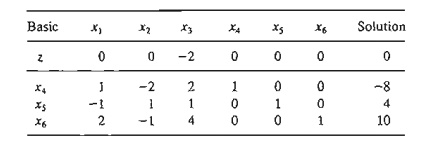
We can solve the problem without the use of any artificial variables or artificial constraints as follows: Remove infeasibility first by applying a version of the dual simplex feasibility condi-tion that selects x₄ as the leaving variable. To determine the entering variable, all we need is a nonbasic variable whose constraint coefficient in the x₄-row is strictly negative. The selection can be done without regard to optimality, because it is nonexistent at this point anyway (compare with the dual optimality condition). In the present example, x₂ has a negative coefficient in the x₄-rowand is selected as the entering variable. The result is the following tableau:

The solution in the preceding tableau is now feasible but nonoptimal, and we can use the primal simplex to determine the optimal solution. In general, had we not restored feasibility in the preceding tableau, we would repeat the procedure as necessary until feasibility is satisfied or there is evidence that the problem has no feasible solution (which happens if a basic variable is negative and all its constraint coefficients are nonnegative). Once feasibility is established, the next step is to pay attention to optimality by applying the proper optimality condition of the pri-mal simplex method.

Remarks. The essence of Example 4.4-2 is that the simplex method is not rigid. The literature abounds with variations of the simplex method (e.g., the primal-dual method, the symmetrical method, the criss-cross method, and the multiplex method) that give the impression that each procedure is different, when, in effect, they all seek a corner point solution, with a slant toward automated computations and, perhaps, computational efficiency.

PROBLEM SET 4.4B

1. The LP model of Problem 4(c), Set 4.4a, has no feasible solution. Show how this condi-tion is detected by the generalized simplex procedure.

2. The LP model of Problem 4(d), Set 4.4a, has no bounded solution. Show how this condi-tion is detected by the generalized sirnplex procedure.