Surface Profiles Determination

Civil - Applied Hydraulic Engineering: Gradually Varied Flow

Surface Profiles Determination

Before one of the profiles discussed above can be decided upon two things must be determined for the channel and flow:

a)    Whether the slope is mild, critical or steep. The normal and critical depths must be calculated for the design discharge

b)    The positions of any  control points  must be established. Control points are points

of known depth or relationship between depth and discharge. Example are weirs, flumes, gates or points where it is known critical flow occurs like at free outfalls, or that the flow is normal depth at some far distance down stream.

Once these control points and depth position has been established the surface profiles can be drawn to join the control points with the insertion of hydraulic jumps where it is necessary to join sub and super critical flows that don't meet at a critical depth.

Below are two examples.

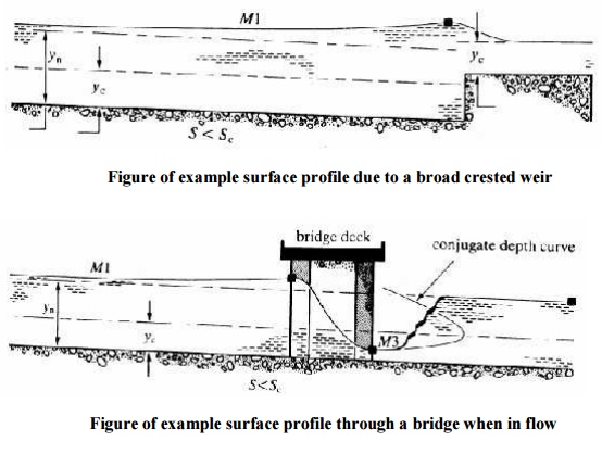
This shows the control point just upstream of a broad crested weir in a channel of mild slope. The resulting curve is an M1.

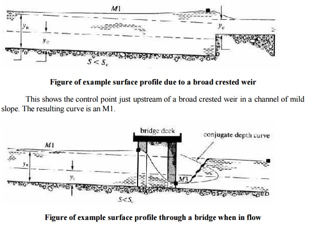
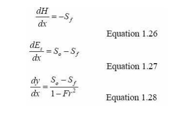
This shows how a bridge may act as a control - particularly under flood conditions. Upstream there is an M1 curve then flow through the bridge is rapidly varied and the depth drops below critical depth so on exit is super critical so a short M3 curve occurs before a hydraulic jump takes the depth back to a sub-critical level. Method of solution of the gradually varied flow equation.

There are three forms of the gradually varied flow equation:

In the past direct and graphical solution methods have been used to solve these, however these method have been superseded by numerical methods which are now be the only method used.

Profile Determination by Numerical method

All (15) of the gradually varied flow profiles shown above may be quickly solved by simple numerical techniques. One computer program can be written to solve most situations.

There are two basic numerical methods that can be used

i.   Direct step - distance from depth

ii.   Standard step method - depth from distance

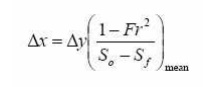
1.The direct step method - distance from depth

This method will calculate (by integrating the gradually varied flow equation) a distance for a given change in surface height.

The equation used is 1.28, which written in finite difference form is

The steps in solution are:

1.  Determine the control depth as the starting point

2.  Decide on the expected curve and depth change if possible

3.  Choose a suitable depth step ?y

4.  Calculate the term in brackets at the 'mean' depth (y initial + ?y/2)

5. Calculate ? x

6.  Repeat 4 and 5 until the appropriate distance / depth changed reached

2.The standard step method - depth from distance

This method will calculate (by integrating the gradually varied flow equation) a depth at a given distance up or downstream.

The equation used is 1.27, which written in finite difference form is

The steps in solution are similar to the direct step method shown above but for each x there is the following iterative step:

1.  Assume a value of depth y (the control depth or the last solution depth)

2.  Calculate the specific energy EsG

3. Calculate S f

4. Calculate ? Es using equation 1.30

5. Calculate  E s(x+ ?x ) s  = E + ? E

6. Repeat until  ?E s (x+ ?x)  = E sG

The Standard step method - alternative form

This method will again calculate a depth at a given distance up or downstream but this time the equation used is 1.26, which written in finite difference form is

The strategy is the same as the first standard step method, with the same necessity to iterate for each step.

2.Graphical Integration Method

This is a simple and straight forward method and is applicable to both prismatic and non prismatic channels of any shape and slope.

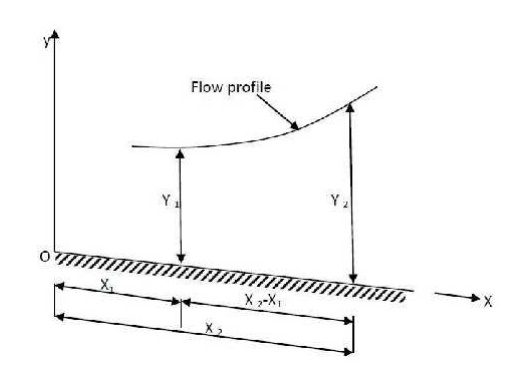
Consider two channel sections at distances x1 and x2 from a chosen reference O as shown in figure above. The depths of flow are y1 and y2 respectively; Let, L= x2-x1, we have

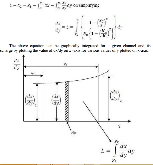
The above equation can be graphically integrated for a given channel and its discharge by plotting the value of dx/dy on x -axis for various values of y plotted on x-axis.

By measuring the area formed by the curve, (the x-axis and the ordinates of dx/dy at y=y1 and y=y2 ) L can be determined. The area can also be determined by computing theordinates dx/dy for different values of y and then, calculating the area between the adjacent ordinates. Summing these areas, one can obtain the desired length L.

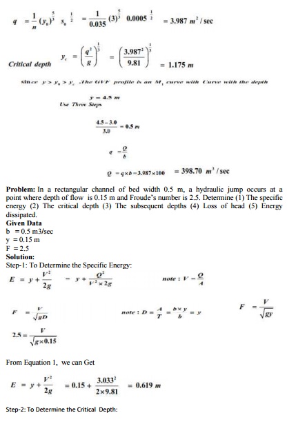
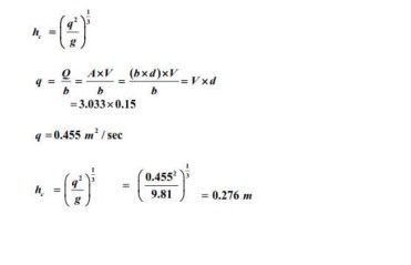
Problem: A river 100 m wide and 3m deep has an average bed slope of 0.0005. Estimate the length of the GVF profile produced by a low weir which raises the water surface just upstream of it by 1.5 m. Assume N = 0.035. Use direct step method with three steps. To estimate the length of the GVF profile