Smith Chart, Solutions Of Problems Using Smith Chart

SMITH CHART, SOLUTIONS OF PROBLEMS USING SMITH CHART

Smith Chart:

The Smith Chart is a fantastic tool for visualizing the impedance of a transmission line and antenna system as a function of frequency. Smith Charts can be used to increase understanding of transmission lines and how they behave from an impedance viewpoint. Smith Charts are also extremely helpful for impedance matching, as we will see. The Smith Chart is used to display a real antenna's impedance when measured on a Vector Network Analyzer (VNA).

Smith Charts were originally developed around 1940 by Phillip Smith as a useful tool for making the equations involved in transmission lines easier to manipulate. See, for instance, the input impedance equation for a load attached to a transmission line of length L and characteristic impedance Z0. With modern computers, the Smith Chart is no longer used to the simplify the calculation of transmission line equatons; however, their value in visualizing the impedance of an antenna or a transmission line has not decreased.

The Smith Chart is shown in Figure 1. A larger version is shown here.

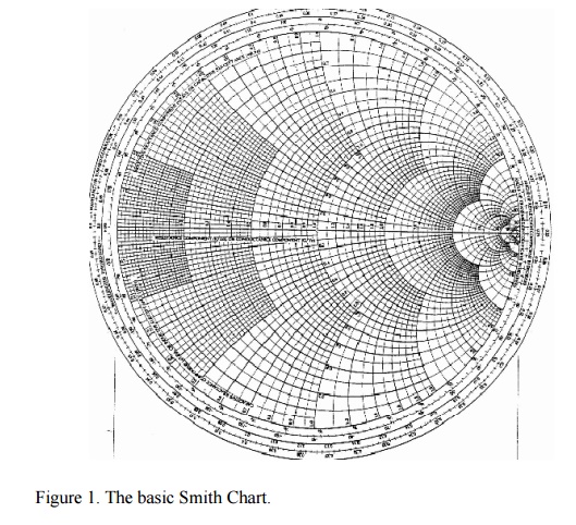
Figure 1 should look a little intimidating, as it appears to be lines going everywhere. There is nothing to fear though. We will build up the Smith Chart from scratch, so that you can understand exactly what all of the lines mean. In fact, we are going to learn an even more complicated version of the Smith Chart known as the immitance Smith Chart, which is twice as complicated, but also twice as useful. But for now, just admire the Smith Chart and its curvy elegance. This section of the antenna theory site will present an intro to the Smith Chart basics.

Smith Chart Tutorial

The Smith Chart displays the complex reflection coefficient, in polar form, for an arbitrary impedance (we'll call the impedance ZL or the load impedance).

For a primer on complex math, click here. Recall that the complex reflection coefficient () for an impedance ZL attached to a transmission line with characteristic impedance Z0 is given by

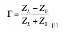
For this tutorial, we will assume Z0 is 50 Ohms, which is often, but not always the case. The complex reflection coefficient, or , must have a magnitude between 0 and 1.

As such, the set of all possible values for must lie within the unit circle:

In Figure 2, plotting the set of all values for the complex reflection coefficient, along the real and imaginary axis. The center of the Smith Chart is the point where the reflection coefficient is zero. That is, this is the only point on the smith chart where no power is reflected by the load impedance.

The outter ring of the Smith Chart is where the magnitude of is equal to 1. This is the black circle in Figure 1. Along this curve, all of the power is reflected by the load impedance.

Normalized Load Impedance

To make the Smith Chart more general and independent of the characteristic impedance Z0 of the transmission line, we will normalize the load impedance ZL by Z0 for all future plots:

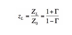
Equation [1] doesn't affect the reflection coefficient tow. It is just a convention that is used everywhere.

Constant Resistance Circles

For a given normalized load impedance zL, we can determine and plot it on the Smith Chart. Now, suppose we have the normalized load impedance given by:

In equation [2], Y is any real number. What would the curve corresponding to equation [2] look like if we plotted it on the Smith Chart for all values of Y? That is, if we plotted z1 = 1 + 0*i, and z1 = 1 + 10*i, z1 = 1 - 5*i, z1 = 1 - .333*i, .... and any possible value for Y that you could think of, what is the resulting curve? The answer is shown in Figure 1:

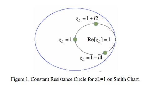
In Figure 1, the outer blue ring represents the boundary of the smith chart. The black curve is a constant resistance circle: this is where all values of z1 = 1 + i*Y will lie on. Several points are plotted along this curve, z1 = 1, z1 = 1 + i*2, and zL = 1 - i*4. Suppose we want to know what the curve z2 = 0.3 + i*Y looks like on the Smith Chart. The result is shown in Figure 2:

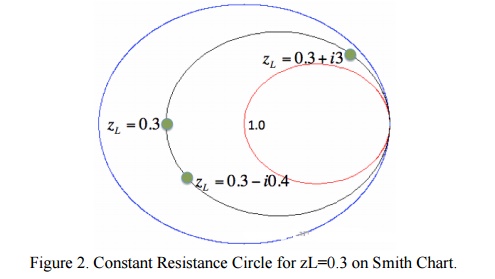
In Figure 2, the black ring represents the set of all impedances where the real part of z2 equals 0.3. A few points along the circle are plotted. We've left the resistance circle of 1.0 in red on the Smith Chart. These circles are called constant resistance curves. The real part of the load impedance is constant along each of these curves. We'll now add several values for the constant resistance, as shown in Figure 3:

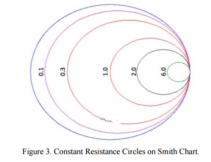
In Figure 3, the zL=0.1 resistance circle has been added in purple. The zL=6 resistance circle has been added in green, and zL=2 resistance circle is in black. look at the set of curves defined by zL = R + iY, where Y is held constant and R varies from 0 to infinity. Since R cannot be negative for antennas or passive devices, we will restrict R to be greater than or equal to zero. As a first example, let zL = R + i. The curve defined by this set of impedances is shown in Figure 1:

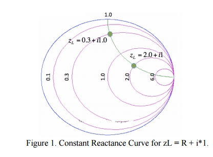
The resulting curve zL = R + i is plotted in green in Figure 1. A few points along the curve are illustrated as well. Observe that zL = 0.3 + i is at the intersection of the Re[zL] = 0.3 circle and the Im[zL]=1 curve. Similarly, observe that the zL = 2 + i point is at the intersection of the Re[zL]=2 circle and the Im[zL]=1 curve. (For a quick reminder of real and imaginary parts of complex numbers, see complex math primer.) The constant reactance curve, defined by Im[zL]=-1 is shown in Figure 2:

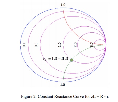
The resulting curve for Im[zL]=-1 is plotted in green in Figure 2. The point zL=1-i is placed on the Smith Chart, which is at the intersection of the Re[zL]=1 circle and the Im[zL]=-1 curve.

An important curve is given by Im[zL]=0. That is, the set of all impedances given by zL = R, where the imaginary part is zero and the real part (the resistance) is greater than or equal to zero. The result is shown in Figure 3:

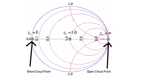
Figure 3. Constant Reactance Curve for zL=R. The reactance curve given by Im[zL]=0 is a straight line across the Smith Chart. There are 3 special points along this curve. On the far left, where zL = 0 + i0, this is the point where the load is a short circuit, and thus the magnitude of is 1, so all power is reflected. In the center of the Smith Chart, we have the point given by zL = 1. At this location, is 0, so the load is exactly matched to the transmission line. No power is reflected at this point.

The point on the far right in Figure 3 is given by zL = infinity. This is the open circuit location. Again, the magnitude of is 1, so all power is reflected at this point, as expected. Finally, we'll add a bunch of constant reactance curves on the Smith Chart, as shown in Figure 4.

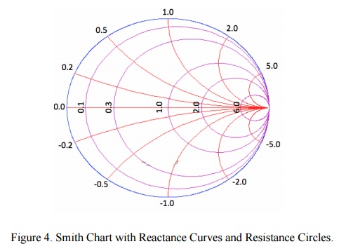
In Figure 4, we added constant reactance curves for Im[zL]=2, Im[zL]=5, Im[zL]=0.2, Im[zL]=0.5, Im[zL]=-2, Im[zL]=-5, Im[zL]=-0.2, and Im[zL] = -0.5. Figure 4 shows the fundamental curves of the Smith Chart.

Applications of smith Chart:

Plotting an impedance

Measurement of VSWR

Measurement of reflection coefficient (magnitude and phase)

Measurement of input impedance of the line

• It is used to find the input impendence and input admittance of the line.

•  The smith chart may also be used for lossy lines and the locus of points on a line then follows a spiral path towards the chart center, due to attenuation.

• In single stub matching.

PROBLEMS:

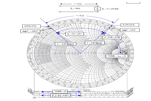
(i). The 0.1λ length line shown has a characteristic impedance of 50 and is terminated with a load impedance of ZL = 5+j25.

(a) Locate zL = ZL/Z0 = 0.1 + j0.5 on the Smith chart.

(b)What is the impedance at l = 0:1λ?

Since we want to move away from the load (i.e., toward the generator), read 0.074 λ on the wavelengths toward generator scale and add l = 0.1 λ to obtain 0.174 λ on the wavelengths toward generator scale.

A radial line from the center of the chart intersects the constant reflection Co-efficient magnitude circle at z = 0.38 + j1.88. Hence Z = zZ0 = 50(0.38 + j1.88) = 19 + 94Ω.

(c) What is the VSWR on the line?

Find VSWR = Zmax = 13 on the horizontal line to the rightof the chart's center. Or use the SWR scale on the chart.

(d) What is ΓL?

From the reflection coefficient scale below the chart,

Find |ΓL| = 0.855. From the angle of reflection coefficient scale on the perimeter of the chart, Find the angle of ΓL=126.5₀.Hence ΓL=0.855e j126.5₀.

(e) What is Γ at l = 0.1λ from the load?

Note that |Γ| =|ΓL|=0.855.Read the angle of the reflection coefficient from the angle of reflection coefficient scale as 55.0₀. Hence ΓL=0.855e j126.5₀.

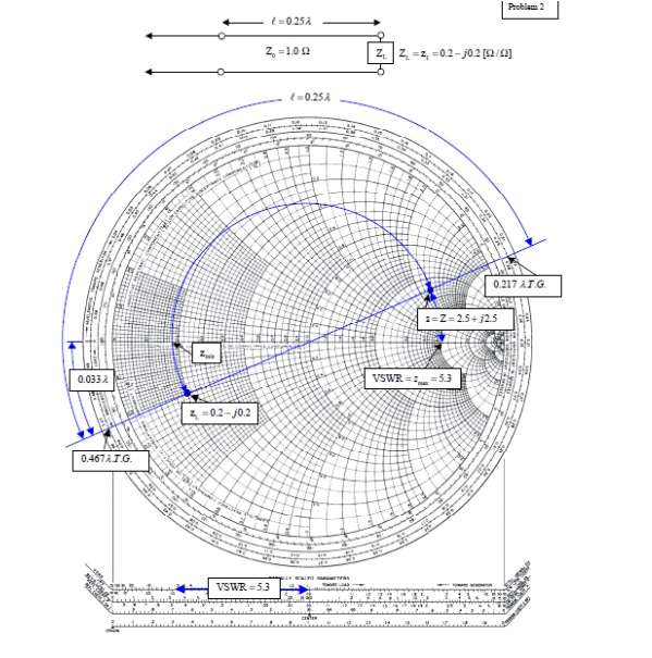
(ii). A transmission line has Z0 = 1.0, ZL = zL = 0.2- j0.2Ω.

(a) What is z at l =λ/4=0.25 λ?

From the chart, read 0:467λfrom the wavelengths to-ward generator scale. Add 0.25λ to obtain 0.717 λ on the wavelengths toward generator scale. This is not on the chart, but since it repeats every half wavelength, it is the same as 0.717 λ – 0.500 λ = 0.217 λ. Drawing a radial line from the center of the chart, we find an intersection with the constant reflection coefficient magnitude circle at z = Z = 2.5 + j2.5.

(b) What is the VSWR on the line?

From the intersection of the constant reflection coefficient circle with the right hand side of the horizontal axis, read VSWR= zmax = 5.3.

(c)  How far from the load is the first voltage minimum?

The voltage minimum occurs at zmin which is at a distance of 0.500λ-0.467λ = 0:033λ from the load. Or read this distance directly on the wavelengths toward load scale.The current minimum occurs at zmax which is a quarter of a wavelength farther down the line or at 0.033λ+0.25λ = 0.283λ from the load.

(iii)           A slotted line measurement yields the following parameter values:

(a) Voltage minima at 9.2 cm and 12.4 cm measured away from the load with the line terminated in a short.

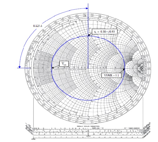
(b) VSWR = 5.1 with the line terminated in the unknown load; a voltage minimum is located 11.6 cm measured away from the load.

What is the normalized line impedance?

Note that this data could have come from either a waveguide or a TEM line measurement. If the transmission system is a waveguide, then the wavelength used is actually the guide wavelength. From the voltage minima on the shorted line, the (guide) wavelength may be determined:

λg/2=12.4cm-9.2 cm=3.2 cm or λg=6.4 λg

Hence the shift in the voltage minimum when the load is replaced by a short is

12.4cm-11.6cm/6.4cm/ λg=0.125 λg

toward the generator. Locate the reflection coefficient magnitude circle by its intersection with zmax = VSWR = 5:1 on the horizontal axis. Then from the voltage minimum opposite zmax, move 0.125 λg toward the generator to find a position an integral number of half-wavelengths from the load. The impedance there is the same as that of the load, zL = 0.38 +j0.93. Alternatively, move 0.5 λg – 0.125 λg = 0.375 λg toward the load to locate the same value.