Chapter: Mathematics (maths) : Numerical Differentiation and Integration
Numerical Differentiation and Integration
NUMERICAL DIFFERENTIATION AND
INTEGRATION
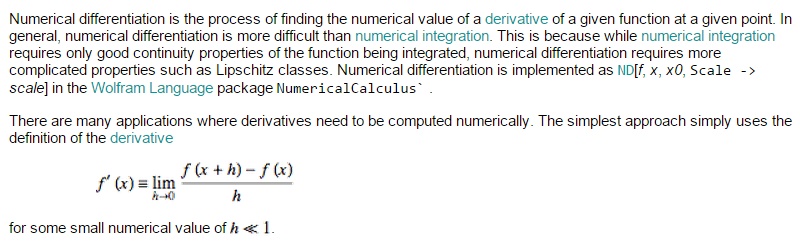
1 Numerical Differentiation Derivatives
using divided differences
Derivatives using finite
Differences
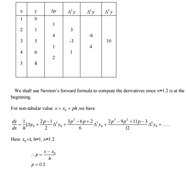
Newton`s forward
interpolation formula
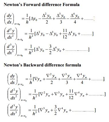
Newton`s Backward
interpolation formula
2 Numerical integration
Trapezoidal Rule
Simpson`s 1/3 Rule
Simpson`s 3/8 Rule
Romberg`s intergration
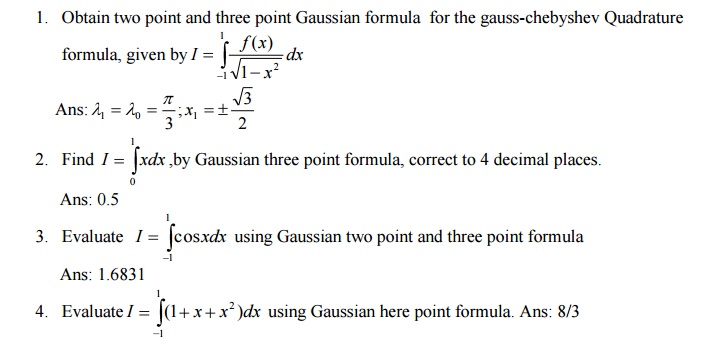
3 Gaussian quadrature
Two Point Gaussian formula
& Three Point Gaussian formula
4 Double integrals
Trapezoidal Rule &
Simpson`s Rule
Introduction
For some particular value of x from the given data (xi,yi), i=1, 2, 3…..n where y=f(x) i explicitly. The interpolation to be used depends on the particular value of x which derivatives are required. If the values of x are not equally spaced, we represent the function by difference formula and the derivatives are obtained. If the values of x are equally spaced, the derivatives are calculated by using Newton’s Forwardinterpolationorformulabackwa.Ifthe derivatives are required at a point near the beginning of the table, we use Newton’sForward interpolation formula and if the derivatives are required at a point near the end of table. We use backward interpolation formula.
1
Derivatives using divided differences
Principle
First fit a polynomial for the given difference data interpolation using Newton ’s divided difference interpolation formula and compute the derivatives for a given x.
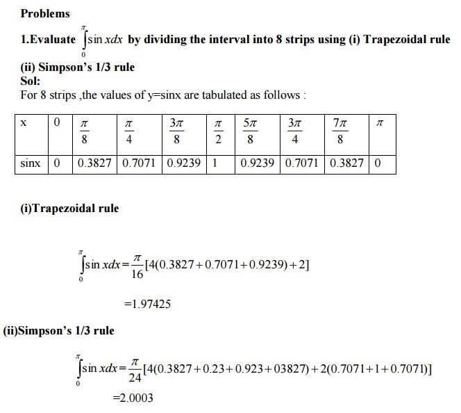
Problems
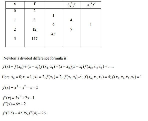
1.Compute f
‘(3.5)
and f ‘’ (4) given that f(0)=2,f(1)=3;f(2)=12 and f(5)=147
Sol:
Divided difference table
2.Find the values f’
(5)and
f’’ (5) using the following data
x 0
2 3 4 7 9
F(x) 4
26 58 112
466 22

Ans:
98 and 34.
1.1 Derivatives using Finite differences
Newton’s
difference Forward Formula
Problems
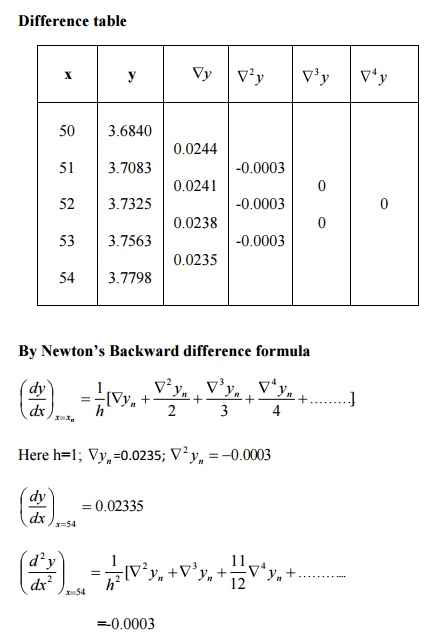
1.Find the first two derivatives of y at
x=54 from the following data
x 50 51 52 53 54
y 3.6840 3.7083 3.7325 3.7563 3.7798

Sol:
Difference table &
2.Find first and second derivatives of
the function at the point x=12 from the following data
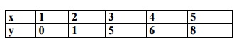
x 1 2 3 4 5
y 0 1 5 6 8
Sol:
Difference table
2
Numerical integration
(Trapezoidal rules, Romberg & Simpson’s integration)
Introduction The process of computing the value of a definite integral from a
set of values (xi,yi),i=0,1,2,x=a;…..xb
of Where the function y=f(x) is called Numerical integration.
Here the function y is replaced by an interpolation
formula involving finite differences and then integrated between the limits a
and b, the value is found.
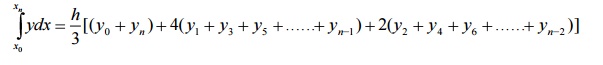
General Quadrature formula for
equidistant ordinates (Newton formula)cote’s
On simplification we obtain
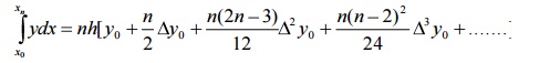
This is the general Quadrature formula
By
putting n=1, Trapezoidal rule is obtained
By
putting n=2, Simpson’s 1/3 rule is derived
By putting n=3,
Simpson’s 3/8 rule is derived.
Note

Simpson’s 1/3
rule
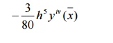
Error in
Simpson’s 1/3 rule

Note
The Error of this formula is of order h5
and the dominant term in the error is given by
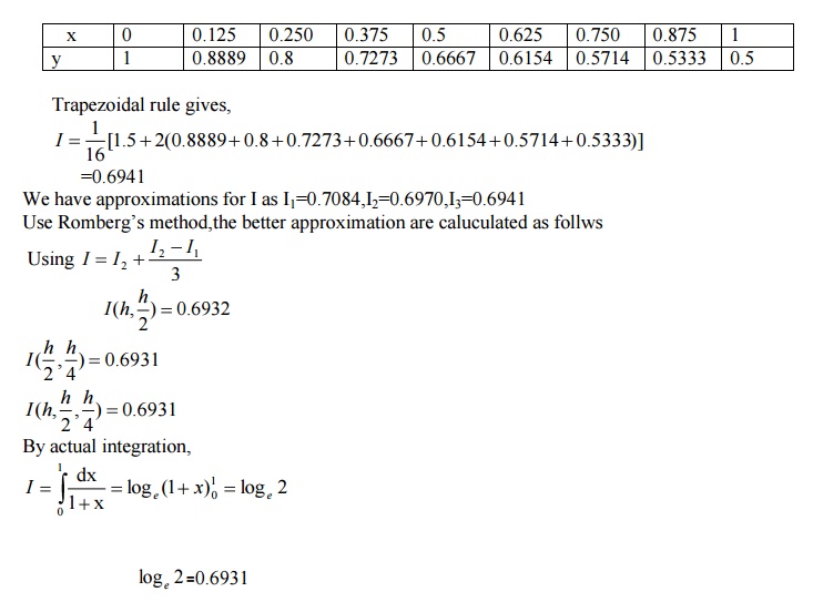
Romberg’s
integration
A simple modification of the Trapezoidal rule can be
used to find a better approximation to the value of an integral. This is based
on the fact that the truncation error of the Trapezoidal rule is nearly
proportional to h2.
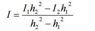
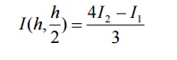
This value of I will be a better approximation than
I1 or I2.This method is called Richardson’s deferred
approach to the limit.
If h1=h and h2=h/2,then we get
3
Gaussian Quadrature
For evaluating the integral
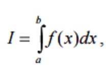
, we derived
some integration rules which require the values of the function at equally
spaced points of the interval. Gauss derived formula which uses the same number
of function values but with the different spacing gives better accuracy.
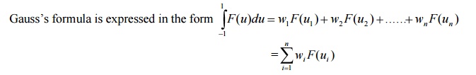
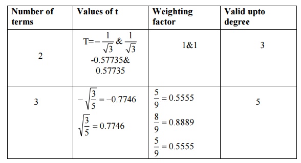
Where wi and u i are called the weights and abscissa
respectively. In this formula, the abscissa and weights are symmetrical with
respect to the middle of the interval. The one-point Gaussian Quadrature
formula is given by
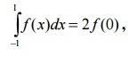
, which
is exact for polynomials of degree upto 1.
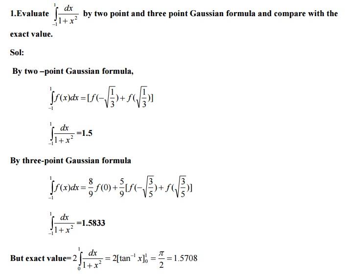
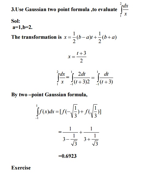
Two point Gaussian formula
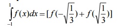
And this is exact for polynomials of degree upto 3.
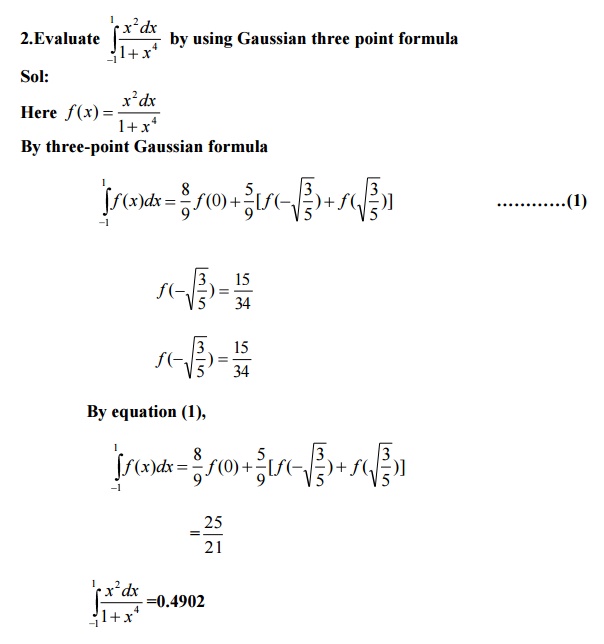
Three point Gaussian formula
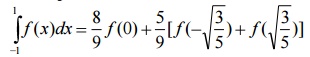
Which is exact for polynomials of degree upto 5
Note:
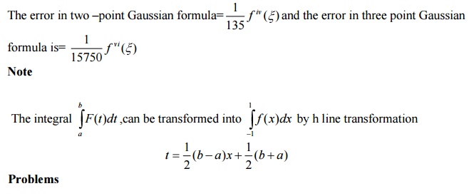
Error terms
The error in two –point Gaussian formula=
4 Double integrals
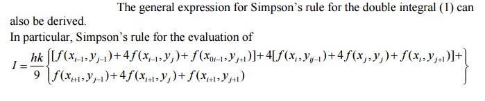
In this session we shall discuss the evaluation of
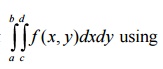
Trapezoidal and Simpson’s rule.
The formulae for the evaluation of a double integral
can be obtained by repeatedly applying the
Trapezoidal and simpson’s
rules.
Consider the integral I
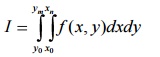
The integration in (1) can be obtained by successive
application of any numerical integration formula with respect to different variables.
Trapezoidal Rule for double integral
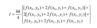
Simpson’s
rule for double
integral
problems
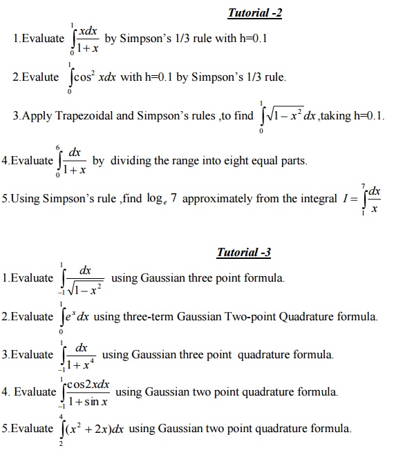
Tutorial problems
Tutorial -1
1.Find the value of f ‘’(3) using divided differences, given data
x 0 1 4 5
F(x) 8 11 68 123
Ans:16
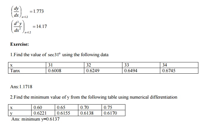
2.Find the first and second derivatives
of the function at the point x=1.2 from the following data
X 1 2 3 4 5
Y 0 1 5 6 8
Ans:14.17
3.A rod is rotating in a plane .The
angle θ ( values of time t (seconds) are given below
t 0 0.2 0.4 0.6 0.8 1.0 1.2
θ 0 0.122 0.493 1.123 2.022 3.220 4.666
Find the angular velocity and angular
acceleration of the rod when t=06 seconds.
Ans:6.7275 radians/sec2.
4.From the table given below ,for what
value of x, y is minimum? Also find this value of y.
X 3 4 5 6 7 8
Y 0.205 0.240 0.25 0.262 0.250 0.224
Ans:5.6875,0.2628
5.Find the first and second derivatives
of y at x=500 from the following data
x 500 510 520 530 540 550
y 6.2146 6.2344 6.2538 6.2792 6.2196 6.3099
Ans:0.002000,-0.0000040
Part
A
1. State the disadvantages of Taylor series method.
Sol:
In the differential equation = f(x,y) the function
f(x,y) may have a complicated
algebraical structure. Then the evaluation of higher
order derivatives may become tedious. This is the demerit of this method.
2. Which is
better Taylor’s method
or R.K met
Sol:
R.K methods do not require prior
calculation of higher derivatives of y(x), as the Taylor method does. Since the
differential equations using in application are often complicated, the
calculation of derivatives may be
difficult. Also R.K formulas involve the computations of f(x,y) at various
positions instead of derivatives and this function occurs in the given
equation.
3. What is a predictor- collector method of solving
a differential equation?
Sol:
predictor-
collector methods are methods which require the values of y at xn, xn-1,
xn-2,…
for computing the values of y at xn+1. We first use a formula to find the values of y at xn+1 and this is known as a predictor formula. The value of y so get is improved or corrected by another formula known as corrector formula.
4. Define a difference Quotient.
Sol:
A difference quotient is the quotient
obtained by dividing the difference between two values of a function, by the
difference between the two corresponding values of the independent.

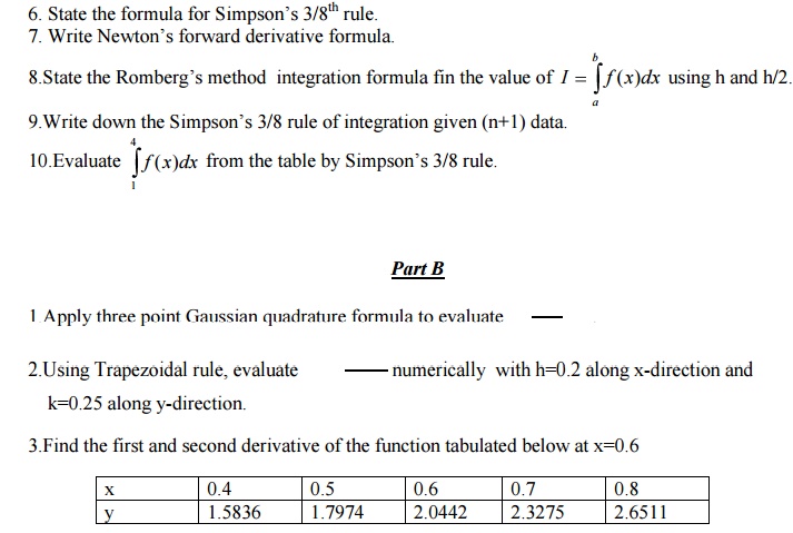
3.Find the first and second derivative of the
function tabulated below at x=0.6
x 0.4 0.5 0.6 0.7 0.8
y 1.5836 1.7974 2.0442 2.3275 2.6511
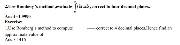
4. Using Romberg’s method dxcorrectto4 decimal to
places compute. Also evaluate the same integral using three –point Gauss
quadrature formula. Comment on the obtained values by comparing with exact
value of the integral which is equal to .
7.Evaluate I=  by dividing the range into ten
equal parts,using
by dividing the range into ten
equal parts,using
(i)Trapezoidal rule
(ii)Simpson’s –third rule.
Verify one your answer with actual integration.
8. Find the first two derivatives of at x=50 and
x=56, for the given table :
x 50 51 52 53 54 55 56
Y=x1/3 3.6840 3.7084 3.7325 3.7325 3.7798 3.8030 3.8259
9.The velocities of a car running on a straight road
at intervals of 2 minutes are given below:
Time(min) 0 2 4 6 8 10 12
Velocity(km/hr) 0 22 30 27 18 7 0
rd
Using
Simpson’s-rulefindthedistance1/3covered by the car.
10. Given
the following data,
find y’(6) and
the
x 0 2 3 4 7 9
Y 4 26 58 112 466 922
Related Topics